TabularExplainer for house-price prediction (regression)

The class TabularExplainer is designed for tabular data, acting as a factory of the supported tabular explainers such as LIME, SHAP and MACE. TabularExplainer provides a unified easy-to-use interface for all the supported explainers. In practice, we recommend applying TabularExplainer to generate explanations instead of using a specific explainer in the package omnixai.explainers.tabular.

# This default renderer is used for sphinx docs only. Please delete this cell in IPython.
import plotly.io as pio
pio.renderers.default = "png"

import numpy as np
import pandas as pd
import sklearn
import sklearn.ensemble
from sklearn.datasets import fetch_california_housing

from omnixai.data.tabular import Tabular
from omnixai.preprocessing.base import Identity
from omnixai.preprocessing.tabular import TabularTransform
from omnixai.explainers.tabular import TabularExplainer
from omnixai.visualization.dashboard import Dashboard

The dataset used in this example is for the house-price prediction (https://scikit-learn.org/stable/modules/generated/sklearn.datasets.fetch_california_housing.html). We recommend using Tabular to represent a tabular dataset that can be constructed from a pandas dataframe or a numpy array. To create a Tabular instance given a pandas dataframe, one needs to specify the dataframe, the categorical feature names (if exists) and the target/label column name (if exists). The package omnixai.preprocessing provides several useful preprocessing functions for a Tabular data.

housing = fetch_california_housing()
df = pd.DataFrame(
    np.concatenate([housing.data, housing.target.reshape((-1, 1))], axis=1),
    columns=list(housing.feature_names) + ['target']
)
tabular_data = Tabular(df, target_column='target')
print(tabular_data)

       MedInc  HouseAge  AveRooms  AveBedrms  Population  AveOccup  Latitude  \
0      8.3252      41.0  6.984127   1.023810       322.0  2.555556     37.88
1      8.3014      21.0  6.238137   0.971880      2401.0  2.109842     37.86
2      7.2574      52.0  8.288136   1.073446       496.0  2.802260     37.85
3      5.6431      52.0  5.817352   1.073059       558.0  2.547945     37.85
4      3.8462      52.0  6.281853   1.081081       565.0  2.181467     37.85
...       ...       ...       ...        ...         ...       ...       ...
20635  1.5603      25.0  5.045455   1.133333       845.0  2.560606     39.48
20636  2.5568      18.0  6.114035   1.315789       356.0  3.122807     39.49
20637  1.7000      17.0  5.205543   1.120092      1007.0  2.325635     39.43
20638  1.8672      18.0  5.329513   1.171920       741.0  2.123209     39.43
20639  2.3886      16.0  5.254717   1.162264      1387.0  2.616981     39.37

       Longitude  target
0        -122.23   4.526
1        -122.22   3.585
2        -122.24   3.521
3        -122.25   3.413
4        -122.25   3.422
...          ...     ...
20635    -121.09   0.781
20636    -121.21   0.771
20637    -121.22   0.923
20638    -121.32   0.847
20639    -121.24   0.894

[20640 rows x 9 columns]

TabularTransform is a special transform designed for tabular data. By default, it converts categorical features into one-hot encoding, and keeps continuous-valued features (if one wants to normalize continuous-valued features, set the parameter cont_transform in TabularTransform to Standard or MinMax). The transform method of TabularTransform will transform a Tabular instance into a numpy array. If the Tabular instance has a target/label column, the last column of the transformed numpy array will be the target/label.

If some other transformations that are not supported in the library are necessary, one can simply convert the Tabular instance into a pandas dataframe by calling Tabular.to_pd() and try different transformations with it.

After data preprocessing, we can train a random forest regressor for this task.

transformer = TabularTransform(
    target_transform=Identity()
).fit(tabular_data)
x = transformer.transform(tabular_data)

x_train, x_test, y_train, y_test = \
    sklearn.model_selection.train_test_split(x[:, :-1], x[:, -1], train_size=0.80)
print('Training data shape: {}'.format(x_train.shape))
print('Test data shape:     {}'.format(x_test.shape))

rf = sklearn.ensemble.RandomForestRegressor(n_estimators=200)
rf.fit(x_train, y_train)
print('MSError when predicting the mean', np.mean((y_train.mean() - y_test) ** 2))
print('Random Forest MSError', np.mean((rf.predict(x_test) - y_test) ** 2))

# Convert the transformed data back to Tabular instances
train_data = transformer.invert(x_train)
test_data = transformer.invert(x_test)

Training data shape: (16512, 8)
Test data shape:     (4128, 8)
MSError when predicting the mean 1.3515599004967849
Random Forest MSError 0.255011664583401

To initialize TabularExplainer, we need to set the following parameters:

• explainers: The names of the explainers to apply, e.g., [“lime”, “shap”, “sensitivity”, “pdp”].

• data: The data used to initialize explainers. data is the training dataset for training the machine learning model. If the training dataset is too large, data can be a subset of it by applying omnixai.sampler.tabular.Sampler.subsample.

• model: The ML model to explain, e.g., a scikit-learn model, a tensorflow model, a pytorch model or a black-box prediction function.

• preprocess: The preprocessing function converting the raw data (a Tabular instance) into the inputs of model.

• postprocess (optional): The postprocessing function transforming the outputs of model to a user-specific form, e.g., the predicted probability for each class. The output of postprocess should be a numpy array.

• mode: The task type, e.g., “classification” or “regression”.

The preprocessing function takes a Tabular instance as its input and outputs the processed features that the ML model consumes. In this example, we simply call transformer.transform. If one uses some special transforms on pandas dataframes, the preprocess function has this kind of format: lambda z: some_transform(z.to_pd()).

preprocess = lambda z: transformer.transform(z)

We are now ready to create a TabularExplainer. params in TabularExplainer allows us to set parameters for each explainer applied here. For example, “kernel_width” for LIME is set to 3.

In this example, LIME and SHAP generate local explanations while PDP (partial dependence plot) and sensitivity analysis generate global explanations. explainers.explain returns the local explanations, and explainers.explain_global returns the global explanations. TabularExplainer hides all the details behind the explainers, so we can simply call these two methods to generate explanations.

# Initialize a TabularExplainer
explainers = TabularExplainer(
    explainers=["lime", "shap", "sensitivity", "pdp", "ale"],
    mode="regression",
    data=train_data,
    model=rf,
    preprocess=preprocess,
    params={
        "lime": {"kernel_width": 3},
        "shap": {"nsamples": 100}
    }
)
# Generate explanations
test_instances = test_data[0:5]
local_explanations = explainers.explain(X=test_instances)
global_explanations = explainers.explain_global(
    params={"pdp": {"features": ["MedInc", "HouseAge", "AveRooms",
                                 "AveBedrms", "Population", "AveOccup",
                                 "Latitude", "Longitude"]}}
)

ipython_plot plots the generated explanations in IPython. Parameter index indicates which instance to plot, e.g., index = 0 means plotting the first instance in test_instances.

index=0
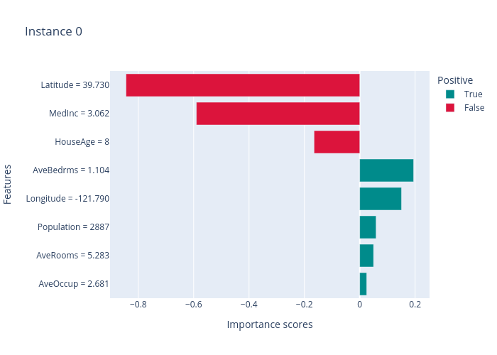
print("LIME results:")
local_explanations["lime"].ipython_plot(index)
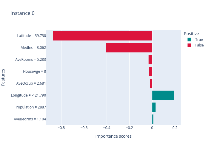
print("SHAP results:")
local_explanations["shap"].ipython_plot(index)
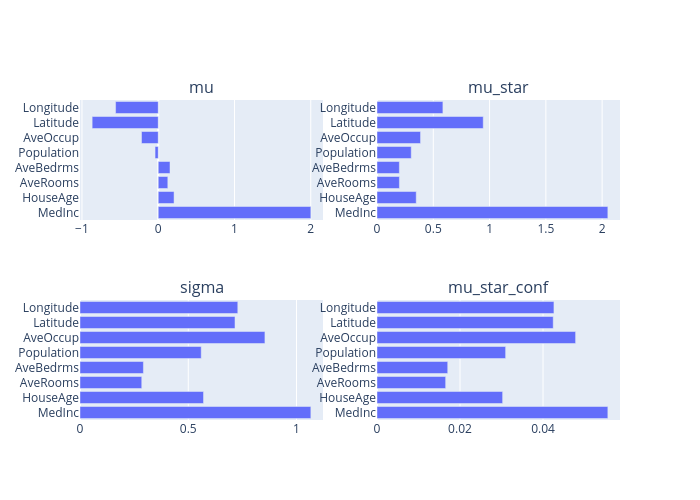
print("Sensitivity results:")
global_explanations["sensitivity"].ipython_plot()
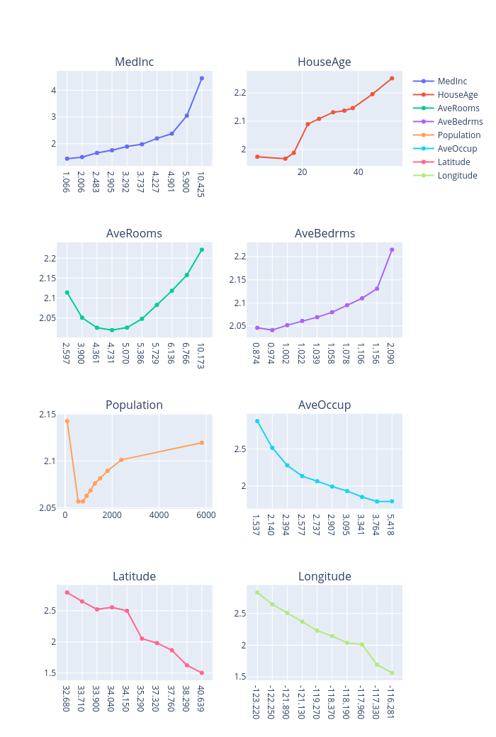
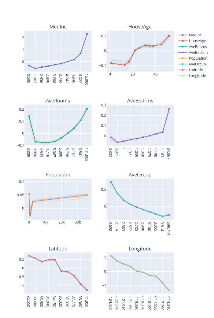
print("PDP results:")
global_explanations["pdp"].ipython_plot()
print("ALE results:")
global_explanations["ale"].ipython_plot()

LIME results:

SHAP results:

Sensitivity results:

PDP results:

ALE results:

Similarly, we create a PredictionAnalyzer for computing performance metrics for this regression task. To initialize PredictionAnalyzer, we set the following parameters:

• mode: The task type, e.g., “classification” or “regression”.

• test_data: The test dataset, which should be a Tabular instance.

• test_targets: The test labels or targets. For regression, test_targets are the observed target values.

• preprocess: The preprocessing function converting the raw data (a Tabular instance) into the inputs of model.

• postprocess (optional): The postprocessing function transforming the outputs of model to a user-specific form. The output of postprocess should be a numpy array.

# Compute metrics
from omnixai.explainers.prediction import PredictionAnalyzer

analyzer = PredictionAnalyzer(
    mode="regression",
    test_data=test_data,
    test_targets=y_test,
    model=rf,
    preprocess=preprocess
)
prediction_explanations = analyzer.explain()

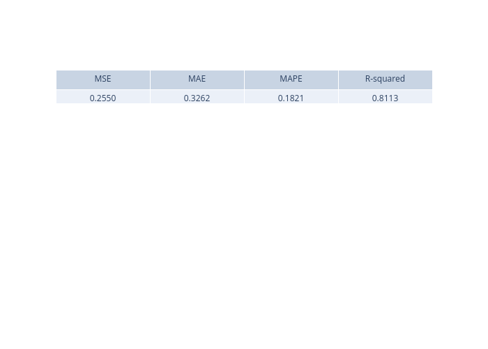
The explain method returns a dict containing multiple metrics:

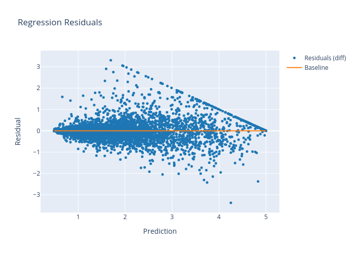
for name, metrics in prediction_explanations.items():
    print(f"{name}:")
    metrics.ipython_plot()

metric:

residual:

Given the generated explanations, we can launch a dashboard (a Dash app) for visualization by setting the test instance, the local explanations, the global explanations, the prediction result analysis, the class names, and additional parameters for visualization (optional).

# Launch a dashboard for visualization
dashboard = Dashboard(
    instances=test_instances,
    local_explanations=local_explanations,
    global_explanations=global_explanations,
    prediction_explanations=prediction_explanations
)
dashboard.show()

Dash is running on http://127.0.0.1:8050/

 * Serving Flask app "omnixai.visualization.dashboard" (lazy loading)
 * Environment: production
   WARNING: This is a development server. Do not use it in a production deployment.
   Use a production WSGI server instead.
 * Debug mode: off

 * Running on http://127.0.0.1:8050/ (Press CTRL+C to quit)