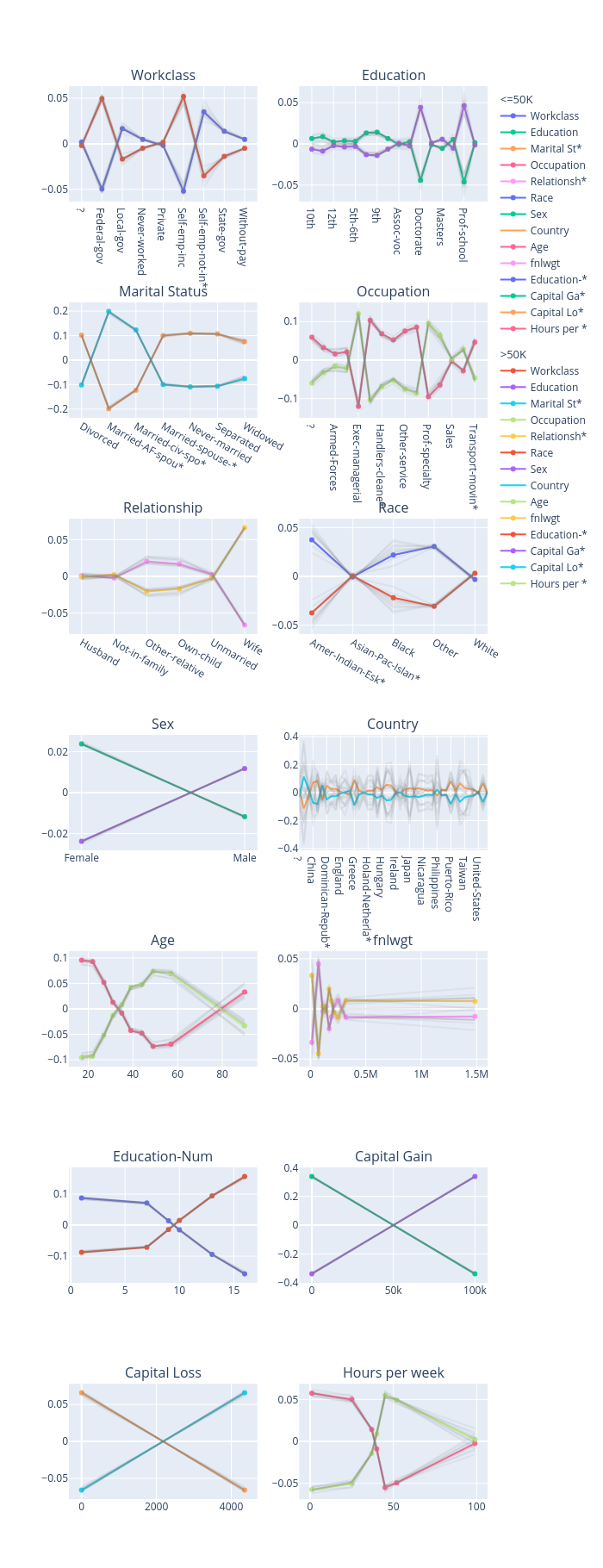
Accumulated local effects (ALE)

# This default renderer is used for sphinx docs only. Please delete this cell in IPython.
import plotly.io as pio
pio.renderers.default = "png"

import os
import sklearn
import xgboost
import numpy as np
import pandas as pd
from omnixai.data.tabular import Tabular
from omnixai.preprocessing.tabular import TabularTransform
from omnixai.explainers.tabular import ALE

The dataset used in this example is for income prediction (https://archive.ics.uci.edu/ml/datasets/adult). We recommend using Tabular to represent a tabular dataset, which can be constructed from a pandas dataframe or a numpy array. To create a Tabular instance given a numpy array, one needs to specify the data, the feature names, the categorical feature names (if exists) and the target/label column name (if exists).

feature_names = [
    "Age", "Workclass", "fnlwgt", "Education",
    "Education-Num", "Marital Status", "Occupation",
    "Relationship", "Race", "Sex", "Capital Gain",
    "Capital Loss", "Hours per week", "Country", "label"
]
data = np.genfromtxt(os.path.join('../data', 'adult.data'), delimiter=', ', dtype=str)
tabular_data = Tabular(
    data,
    feature_columns=feature_names,
    categorical_columns=[feature_names[i] for i in [1, 3, 5, 6, 7, 8, 9, 13]],
    target_column='label'
)

TabularTransform is a special transform designed for tabular data. By default, it converts categorical features into one-hot encoding, and keeps continuous-valued features (if one wants to normalize continuous-valued features, set the parameter cont_transform in TabularTransform to Standard or MinMax). The transform method of TabularTransform will transform a Tabular instance into a numpy array. If the Tabular instance has a target/label column, the last column of the transformed numpy array will be the target/label.

If one wants some other transformations that are not supported in the library, one can simply convert the Tabular instance into a pandas dataframe by calling Tabular.to_pd() and try different transformations with it.

After data preprocessing, we can train a XGBoost classifier for this task (one may try other classifiers).

np.random.seed(1)
transformer = TabularTransform().fit(tabular_data)
class_names = transformer.class_names
x = transformer.transform(tabular_data)
train, test, train_labels, test_labels = \
    sklearn.model_selection.train_test_split(x[:, :-1], x[:, -1], train_size=0.80)
print('Training data shape: {}'.format(train.shape))
print('Test data shape:     {}'.format(test.shape))

gbtree = xgboost.XGBClassifier(n_estimators=300, max_depth=5)
gbtree.fit(train, train_labels)
print('Test accuracy: {}'.format(
    sklearn.metrics.accuracy_score(test_labels, gbtree.predict(test))))

Training data shape: (26048, 108)
Test data shape:     (6513, 108)
Test accuracy: 0.8668816213726394

The prediction function takes a Tabular instance as its inputs, and outputs the class probabilities for classification tasks or the estimated values for regression tasks. In this example, we simply call transformer.transform to do data preprocessing followed by the prediction function of gbtree.

predict_function=lambda z: gbtree.predict_proba(transformer.transform(z))

To initialize an ALE explainer, we need to set:

• training_data: The data used to initialize the explainer. training_data can be the training dataset for training the machine learning model. If the training dataset is too large, training_data can be a subset of it by applying omnixai.sampler.tabular.Sampler.subsample.

• predict_function: The prediction function corresponding to the model.

• mode: The task type, e.g., “classification” or “regression”.

explainer = ALE(
    training_data=tabular_data,
    predict_function=predict_function
)

explanations = explainer.explain()
explanations.ipython_plot(class_names=class_names)