MACE counterfactual explanation for income prediction
This is an example of the Model-Agnostic Counterfactual Explanation (MACE) developed by Yang et al. If using this explainer, please cite our paper “MACE: An Efficient Model-Agnostic Framework for Counterfactual Explanation”. MACE supports black-box models for classification tasks where input features can either be categorical or continuous-valued, and generates diverse counterfactual examples.
[1]:
# This default renderer is used for sphinx docs only. Please delete this cell in IPython.
import plotly.io as pio
pio.renderers.default = "png"
[2]:
import os
import sklearn
import xgboost
import numpy as np
import pandas as pd
from omnixai.data.tabular import Tabular
from omnixai.preprocessing.tabular import TabularTransform
from omnixai.explainers.tabular import MACEExplainer
The dataset used in this example is for income prediction (https://archive.ics.uci.edu/ml/datasets/adult). We recommend using Tabular to represent a tabular dataset, which can be constructed from a pandas dataframe or a numpy array. To create a Tabular instance given a numpy array, one needs to specify the data, the feature names, the categorical feature names (if exists) and the target/label column name (if exists).
[3]:
feature_names = [
    "Age", "Workclass", "fnlwgt", "Education",
    "Education-Num", "Marital Status", "Occupation",
    "Relationship", "Race", "Sex", "Capital Gain",
    "Capital Loss", "Hours per week", "Country", "label"
]
data = np.genfromtxt(os.path.join('../data', 'adult.data'), delimiter=', ', dtype=str)
tabular_data = Tabular(
    data,
    feature_columns=feature_names,
    categorical_columns=[feature_names[i] for i in [1, 3, 5, 6, 7, 8, 9, 13]],
    target_column='label'
)
print(tabular_data)
      Age         Workclass  fnlwgt   Education Education-Num  \
0      39         State-gov   77516   Bachelors            13
1      50  Self-emp-not-inc   83311   Bachelors            13
2      38           Private  215646     HS-grad             9
3      53           Private  234721        11th             7
4      28           Private  338409   Bachelors            13
...    ..               ...     ...         ...           ...
32556  27           Private  257302  Assoc-acdm            12
32557  40           Private  154374     HS-grad             9
32558  58           Private  151910     HS-grad             9
32559  22           Private  201490     HS-grad             9
32560  52      Self-emp-inc  287927     HS-grad             9

           Marital Status         Occupation   Relationship   Race     Sex  \
0           Never-married       Adm-clerical  Not-in-family  White    Male
1      Married-civ-spouse    Exec-managerial        Husband  White    Male
2                Divorced  Handlers-cleaners  Not-in-family  White    Male
3      Married-civ-spouse  Handlers-cleaners        Husband  Black    Male
4      Married-civ-spouse     Prof-specialty           Wife  Black  Female
...                   ...                ...            ...    ...     ...
32556  Married-civ-spouse       Tech-support           Wife  White  Female
32557  Married-civ-spouse  Machine-op-inspct        Husband  White    Male
32558             Widowed       Adm-clerical      Unmarried  White  Female
32559       Never-married       Adm-clerical      Own-child  White    Male
32560  Married-civ-spouse    Exec-managerial           Wife  White  Female

      Capital Gain Capital Loss Hours per week        Country  label
0             2174            0             40  United-States  <=50K
1                0            0             13  United-States  <=50K
2                0            0             40  United-States  <=50K
3                0            0             40  United-States  <=50K
4                0            0             40           Cuba  <=50K
...            ...          ...            ...            ...    ...
32556            0            0             38  United-States  <=50K
32557            0            0             40  United-States   >50K
32558            0            0             40  United-States  <=50K
32559            0            0             20  United-States  <=50K
32560        15024            0             40  United-States   >50K

[32561 rows x 15 columns]
TabularTransform is a special transform designed for tabular data. By default, it converts categorical features into one-hot encoding, and keeps continuous-valued features (if one wants to normalize continuous-valued features, set the parameter cont_transform in TabularTransform to Standard or MinMax). The transform method of TabularTransform will transform a Tabular instance into a numpy array. If the Tabular instance has a target/label column, the last
column of the transformed numpy array will be the target/label.
If some other transformations that are not supported in the library are necessary, one can simply convert the Tabular instance into a pandas dataframe by calling Tabular.to_pd() and try different transformations with it.
After data preprocessing, we can train a XGBoost classifier for this task (one may try other classifiers).
[4]:
np.random.seed(1)
transformer = TabularTransform().fit(tabular_data)
class_names = transformer.class_names
x = transformer.transform(tabular_data)
train, test, labels_train, labels_test = \
    sklearn.model_selection.train_test_split(x[:, :-1], x[:, -1], train_size=0.80)
print('Training data shape: {}'.format(train.shape))
print('Test data shape:     {}'.format(test.shape))

gbtree = xgboost.XGBClassifier(n_estimators=300, max_depth=5)
gbtree.fit(train, labels_train)
print('Test accuracy: {}'.format(
    sklearn.metrics.accuracy_score(labels_test, gbtree.predict(test))))
Training data shape: (26048, 108)
Test data shape:     (6513, 108)
Test accuracy: 0.8668816213726394
The prediction function takes a Tabular instance as its inputs, and outputs the class probabilities or logits for classification tasks or the estimated values for regression tasks. In this example, we simply call transformer.transform to do data preprocessing followed by the prediction function of gbtree.
[5]:
predict_function=lambda z: gbtree.predict_proba(transformer.transform(z))
To initialize a MACE explainer, we need to set:
training_data: The data used to initialize a MACE explainer.training_datacan be the training dataset for training the machine learning model. If the training dataset is too large,training_datacan be a subset of it by applyingomnixai.sampler.tabular.Sampler.subsample.predict_function: The prediction function corresponding to the model.ignored_features: The features ignored in generating counterfactual examples, i.e., those features are fixed.
In this example, we set ignored_features=["Sex", "Race", "Relationship", "Capital Loss"], meaning that the generated counterfactual examples don’t change the values of these features.
[6]:
explainer = MACEExplainer(
    training_data=tabular_data,
    predict_function=predict_function,
    ignored_features=["Sex", "Race", "Relationship", "Capital Loss"]
)
test_instances = tabular_data.remove_target_column()[0:5]
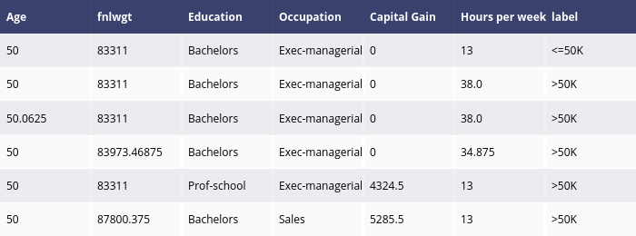
MACE generates local explanations, e.g. explainer.explain is called given the test instances. ipython_plot plots the generated explanations in IPython. Parameter index indicates which instance to plot, e.g., index = 1 means plotting the second instance in test_instances.
[7]:
explanations = explainer.explain(test_instances)
explanations.ipython_plot(index=1, class_names=class_names)