How to Use Anomaly Detectors in Merlion
This notebook will guide you through using all the key features of anomaly detectors in Merlion. Specifically, we will explain
Initializing an anomaly detection model (including ensembles)
Training the model
Producing a series of anomaly scores with the model
Quantitatively evaluating the model
Visualizing the model’s predictions
Saving and loading a trained model
Simulating the live deployment of a model using a
TSADEvaluator
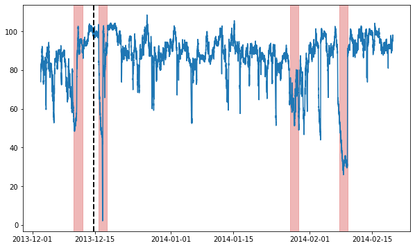
We will be using a single example time series for this whole notebook. We load and visualize it now:
[1]:
import matplotlib.pyplot as plt
import numpy as np

from merlion.plot import plot_anoms
from merlion.utils import TimeSeries
from ts_datasets.anomaly import NAB

np.random.seed(1234)

# This is a time series with anomalies in both the train and test split.
# time_series and metadata are both time-indexed pandas DataFrames.
time_series, metadata = NAB(subset="realKnownCause")[3]

# Visualize the full time series
fig = plt.figure(figsize=(10, 6))
ax = fig.add_subplot(111)
ax.plot(time_series)

# Label the train/test split with a dashed line & plot anomalies
ax.axvline(metadata[metadata.trainval].index[-1], ls="--", lw=2, c="k")
plot_anoms(ax, TimeSeries.from_pd(metadata.anomaly))
Time series /Users/isenilov/dev/Merlion/data/nab/realKnownCause/ec2_request_latency_system_failure.csv (index 2) has timestamp duplicates. Kept first values.
Time series /Users/isenilov/dev/Merlion/data/nab/realKnownCause/machine_temperature_system_failure.csv (index 3) has timestamp duplicates. Kept first values.
[2]:
from merlion.utils import TimeSeries

# Get training split
train = time_series[metadata.trainval]
train_data = TimeSeries.from_pd(train)
train_labels = TimeSeries.from_pd(metadata[metadata.trainval].anomaly)

# Get testing split
test = time_series[~metadata.trainval]
test_data = TimeSeries.from_pd(test)
test_labels = TimeSeries.from_pd(metadata[~metadata.trainval].anomaly)
Model Initialization
In this notebook, we will use three different anomaly detection models:
Isolation Forest (a classic anomaly detection model)
WindStats (an in-house model that divides each week into windows of a specified size, and compares time series values to the historical values in the appropriate window)
Prophet (Facebook’s popular forecasting model, adapted for anomaly detection.
Let’s start by initializing each of them:
[3]:
# Import models & configs
from merlion.models.anomaly.isolation_forest import IsolationForest, IsolationForestConfig
from merlion.models.anomaly.windstats import WindStats, WindStatsConfig
from merlion.models.anomaly.forecast_based.prophet import ProphetDetector, ProphetDetectorConfig

# Import a post-rule for thresholding
from merlion.post_process.threshold import AggregateAlarms

# Import a data processing transform
from merlion.transform.moving_average import DifferenceTransform

# All models are initialized using the syntax ModelClass(config), where config
# is a model-specific configuration object. This is where you specify any
# algorithm-specific hyperparameters, any data pre-processing transforms, and
# the post-rule you want to use to post-process the anomaly scores (to reduce
# noisiness when firing alerts).

# We initialize isolation forest using the default config
config1 = IsolationForestConfig()
model1  = IsolationForest(config1)

# We use a WindStats model that splits each week into windows of 60 minutes
# each. Anomaly scores in Merlion correspond to z-scores. By default, we would
# like to fire an alert for any 4-sigma event, so we specify a threshold rule
# which achieves this.
config2 = WindStatsConfig(wind_sz=60, threshold=AggregateAlarms(alm_threshold=4))
model2  = WindStats(config2)

# Prophet is a popular forecasting algorithm. Here, we specify that we would like
# to pre-processes the input time series by applying a difference transform,
# before running the model on it.
config3 = ProphetDetectorConfig(transform=DifferenceTransform())
model3  = ProphetDetector(config3)
Now that we have initialized the individual models, we will also combine them in an ensemble. We set this ensemble’s detection threshold to fire alerts for 4-sigma events (the same as WindStats).
[4]:
from merlion.models.ensemble.anomaly import DetectorEnsemble, DetectorEnsembleConfig

ensemble_config = DetectorEnsembleConfig(threshold=AggregateAlarms(alm_threshold=4))
ensemble = DetectorEnsemble(config=ensemble_config, models=[model1, model2, model3])
Model Training
All anomaly detection models (and ensembles) share the same API for training. The train() method returns the model’s predicted anomaly scores on the training data. Note that you may optionally specify configs that modify the protocol used to train the model’s post-rule! You may optionally specify ground truth anomaly labels as well (if you have them), but they are not needed. We give examples of all these behaviors below.
[5]:
from merlion.evaluate.anomaly import TSADMetric

# Train IsolationForest in the default way, using the ground truth anomaly labels
# to set the post-rule's threshold
print(f"Training {type(model1).__name__}...")
train_scores_1 = model1.train(train_data=train_data, anomaly_labels=train_labels)

# Train WindStats completely unsupervised (this retains our anomaly detection
# default anomaly detection threshold of 4)
print(f"\nTraining {type(model2).__name__}...")
train_scores_2 = model2.train(train_data=train_data, anomaly_labels=None)

# Train Prophet with the ground truth anomaly labels, with a post-rule
# trained to optimize Precision score
print(f"\nTraining {type(model3).__name__}...")
post_rule_train_config_3 = dict(metric=TSADMetric.F1)
train_scores_3 = model3.train(
    train_data=train_data, anomaly_labels=train_labels,
    post_rule_train_config=post_rule_train_config_3)

# We consider an unsupervised ensemble, which combines the anomaly scores
# returned by the models & sets a static anomaly detection threshold of 3.
print("\nTraining ensemble...")
ensemble_post_rule_train_config = dict(metric=None)
train_scores_e = ensemble.train(
    train_data=train_data, anomaly_labels=train_labels,
    post_rule_train_config=ensemble_post_rule_train_config,
)

print("Done!")
Training IsolationForest...
INFO:merlion.post_process.threshold:Threshold 3.2263 achieves F1=0.5000.
INFO:prophet:Disabling yearly seasonality. Run prophet with yearly_seasonality=True to override this.
INFO:prophet:Disabling weekly seasonality. Run prophet with weekly_seasonality=True to override this.
Training WindStats...

Training ProphetDetector...
INFO:merlion.post_process.threshold:Threshold 3.2263 achieves F1=0.6667.
Training ensemble...
INFO:prophet:Disabling yearly seasonality. Run prophet with yearly_seasonality=True to override this.
INFO:prophet:Disabling weekly seasonality. Run prophet with weekly_seasonality=True to override this.
Done!
Model Inference
There are two ways to invoke an anomaly detection model: model.get_anomaly_score() returns the model’s raw anomaly scores, while model.get_anomaly_label() returns the model’s post-processed anomaly scores. The post-processing calibrates the anomaly scores to be interpretable as z-scores, and it also sparsifies them such that any nonzero values should be treated as an alert that a particular timestamp is anomalous.
[6]:
# Here is a full example for the first model, IsolationForest
scores_1 = model1.get_anomaly_score(test_data)
scores_1_df = scores_1.to_pd()
print(f"{type(model1).__name__}.get_anomaly_score() nonzero values (raw)")
print(scores_1_df[scores_1_df.iloc[:, 0] != 0])
print()

labels_1 = model1.get_anomaly_label(test_data)
labels_1_df = labels_1.to_pd()
print(f"{type(model1).__name__}.get_anomaly_label() nonzero values (post-processed)")
print(labels_1_df[labels_1_df.iloc[:, 0] != 0])
print()

print(f"{type(model1).__name__} fires {(labels_1_df.values != 0).sum()} alarms")
print()

print("Raw scores at the locations where alarms were fired:")
print(scores_1_df[labels_1_df.iloc[:, 0] != 0])
print("Post-processed scores are interpretable as z-scores")
print("Raw scores are challenging to interpret")
IsolationForest.get_anomaly_score() nonzero values (raw)
                     anom_score
2013-12-14 16:55:00    0.424103
2013-12-14 17:00:00    0.418938
2013-12-14 17:05:00    0.484891
2013-12-14 17:10:00    0.500257
2013-12-14 17:15:00    0.449213
...                         ...
2014-02-19 15:05:00    0.419456
2014-02-19 15:10:00    0.415807
2014-02-19 15:15:00    0.406724
2014-02-19 15:20:00    0.427094
2014-02-19 15:25:00    0.428348

[19279 rows x 1 columns]

IsolationForest.get_anomaly_label() nonzero values (post-processed)
                     anom_score
2013-12-16 16:00:00    3.251397
2013-12-16 18:35:00    3.681691
2013-12-27 19:25:00    3.914430
2013-12-27 23:20:00    3.260543
2013-12-28 04:15:00    3.738462
2013-12-28 06:20:00    3.303482
2014-01-02 10:00:00    3.233514
2014-01-05 17:50:00    3.791805
2014-01-12 09:25:00    3.535895
2014-01-13 10:05:00    3.314500
2014-01-16 12:50:00    3.850349
2014-01-24 12:50:00    4.170855
2014-01-27 17:45:00    3.537919
2014-01-28 22:00:00    3.451974
2014-01-30 23:40:00    3.550075
2014-02-02 23:45:00    3.359105
2014-02-03 11:55:00    4.175556
2014-02-05 05:10:00    3.675433
2014-02-09 11:55:00    4.005116
2014-02-13 19:15:00    3.247573

IsolationForest fires 20 alarms

Raw scores at the locations where alarms were fired:
                     anom_score
2013-12-16 16:00:00    0.701491
2013-12-16 18:35:00    0.772563
2013-12-27 19:25:00    0.810997
2013-12-27 23:20:00    0.702972
2013-12-28 04:15:00    0.781997
2013-12-28 06:20:00    0.709952
2014-01-02 10:00:00    0.698602
2014-01-05 17:50:00    0.790835
2014-01-12 09:25:00    0.748293
2014-01-13 10:05:00    0.711750
2014-01-16 12:50:00    0.800493
2014-01-24 12:50:00    0.852493
2014-01-27 17:45:00    0.748630
2014-01-28 22:00:00    0.734366
2014-01-30 23:40:00    0.750652
2014-02-02 23:45:00    0.719052
2014-02-03 11:55:00    0.853260
2014-02-05 05:10:00    0.771522
2014-02-09 11:55:00    0.825713
2014-02-13 19:15:00    0.700873
Post-processed scores are interpretable as z-scores
Raw scores are challenging to interpret
The same API is shared for all models, including ensembles.
[7]:
scores_2 = model2.get_anomaly_score(test_data)
labels_2 = model2.get_anomaly_label(test_data)
[8]:
scores_3 = model3.get_anomaly_score(test_data)
labels_3 = model3.get_anomaly_label(test_data)
[9]:
scores_e = ensemble.get_anomaly_score(test_data)
labels_e = ensemble.get_anomaly_label(test_data)
Quantitative Evaluation
It is fairly transparent to visualize a model’s predicted anomaly scores and also quantitatively evaluate its anomaly labels. For evaluation, we use specialized definitions of precision, recall, and F1 as revised point-adjusted metrics (see the technical report for more details). We also consider the mean time to detect anomalies.
In general, you may use the TSADMetric enum to compute evaluation metrics for a time series using the syntax
TSADMetric.<metric_name>.value(ground_truth=ground_truth, predict=anomaly_labels)
where <metric_name> is the name of the evaluation metric (see the API docs for details and more options), ground_truth is a time series of ground truth anomaly labels, and anomaly_labels is the output of model.get_anomaly_label().
[10]:
from merlion.evaluate.anomaly import TSADMetric

for model, labels in [(model1, labels_1), (model2, labels_2), (model3, labels_3), (ensemble, labels_e)]:
    print(f"{type(model).__name__}")
    precision = TSADMetric.Precision.value(ground_truth=test_labels, predict=labels)
    recall = TSADMetric.Recall.value(ground_truth=test_labels, predict=labels)
    f1 = TSADMetric.F1.value(ground_truth=test_labels, predict=labels)
    mttd = TSADMetric.MeanTimeToDetect.value(ground_truth=test_labels, predict=labels)
    print(f"Precision: {precision:.4f}")
    print(f"Recall:    {recall:.4f}")
    print(f"F1:        {f1:.4f}")
    print(f"MTTD:      {mttd}")
    print()
IsolationForest
Precision: 0.1667
Recall:    1.0000
F1:        0.2857
MTTD:      0 days 23:31:40

WindStats
Precision: 0.2500
Recall:    0.6667
F1:        0.3636
MTTD:      1 days 10:25:00

ProphetDetector
Precision: 0.3750
Recall:    1.0000
F1:        0.5455
MTTD:      1 days 00:03:20

DetectorEnsemble
Precision: 0.4000
Recall:    0.6667
F1:        0.5000
MTTD:      1 days 10:25:00
Since the individual models are trained to optimize F1 directly, they all have low precision, high recall, and a mean time to detect of around 1 day. However, by instead training the individual models to optimize precision, and training a model combination unit to optimize F1, we are able to greatly increase the precision and F1 score, at the cost of a lower recall and higher mean time to detect.
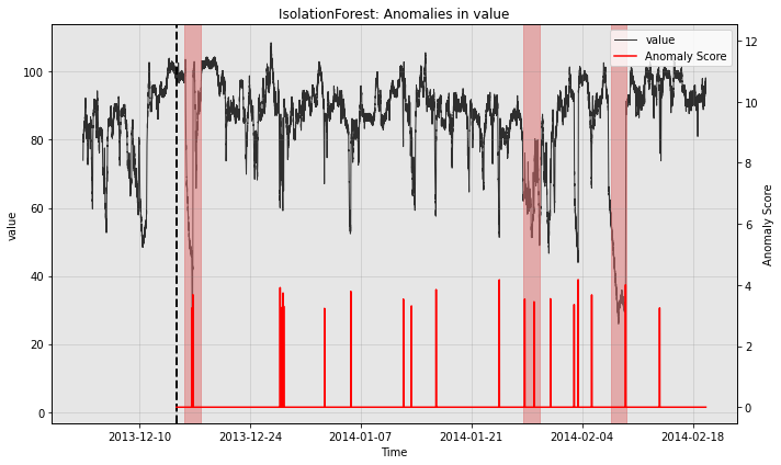
Model Visualization
Let’s now visualize the model predictions that led to these outcomes. The option filter_scores=True means that we want to plot the post-processed anomaly scores (i.e. returned by model.get_anomaly_label()). You may instead specify filter_scores=False to visualize the raw anomaly scores.
[11]:
for model in [model1, model2, model3]:
    print(type(model).__name__)
    fig, ax = model.plot_anomaly(
        time_series=test_data, time_series_prev=train_data,
        filter_scores=True, plot_time_series_prev=True)
    plot_anoms(ax=ax, anomaly_labels=test_labels)
    plt.show()
    print()
IsolationForest
WindStats

ProphetDetector
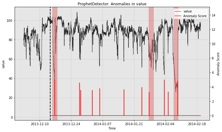
So all the individual models generate quite a few false positives. Let’s see how the ensemble does:
[12]:
fig, ax = ensemble.plot_anomaly(
    time_series=test_data, time_series_prev=train_data,
    filter_scores=True, plot_time_series_prev=True)
plot_anoms(ax=ax, anomaly_labels=test_labels)
plt.show()
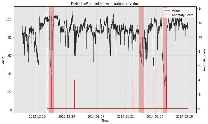
So the ensemble misses one of the three anomalies in the test split, but it also greatly reduces the number of false positives relative to the other models.
Saving & Loading Models
All models have a save() method and load() class method. Models may also be loaded with the assistance of the ModelFactory, which works for arbitrary models. The save() method creates a new directory at the specified path, where it saves a json file representing the model’s config, as well as a binary file for the model’s state.
We will demonstrate these behaviors using our IsolationForest model (model1) for concreteness. Note that the config explicitly tracks the transform (to pre-process the data), the calibrator (to transform raw anomaly scores into z-scores), the thresholding rule (to sparsify the calibrated anomaly scores).
[13]:
import json
import os
import pprint
from merlion.models.factory import ModelFactory

# Save the model
os.makedirs("models", exist_ok=True)
path = os.path.join("models", "isf")
model1.save(path)

# Print the config saved
pp = pprint.PrettyPrinter()
with open(os.path.join(path, "config.json")) as f:
    print(f"{type(model1).__name__} Config")
    pp.pprint(json.load(f))

# Load the model using Prophet.load()
model2_loaded = IsolationForest.load(dirname=path)

# Load the model using the ModelFactory
model2_factory_loaded = ModelFactory.load(name="IsolationForest", model_path=path)
IsolationForest Config
{'calibrator': {'abs_score': True,
                'anchors': [[0.38992633996347176, 0.0],
                            [0.4187750781361715, 0.5],
                            [0.445336977389891, 1.0],
                            [0.47974261897360404, 1.5],
                            [0.5271631189090943, 2.0],
                            [0.8301789920204418, 4.032894437734716],
                            [1.0, 5.032894437734716]],
                'max_score': 1.0,
                'name': 'AnomScoreCalibrator'},
 'dim': 1,
 'enable_calibrator': True,
 'enable_threshold': True,
 'max_n_samples': 1.0,
 'n_estimators': 100,
 'threshold': {'abs_score': True,
               'alm_suppress_minutes': 120,
               'alm_threshold': 3.2263155501877727,
               'alm_window_minutes': 60,
               'min_alm_in_window': 2,
               'name': 'AggregateAlarms'},
 'transform': {'name': 'TransformSequence',
               'transforms': [{'name': 'DifferenceTransform'},
                              {'multivar_skip': True,
                               'name': 'Shingle',
                               'size': 2,
                               'stride': 1}]}}
We can do the same exact thing with ensembles! Note that the ensemble stores its underlying models in a nested structure. This is all reflected in the config.
[14]:
# Save the ensemble
path = os.path.join("models", "ensemble")
ensemble.save(path)

# Print the config saved. Note that we've saved all individual models,
# and their paths are specified under the model_paths key.
pp = pprint.PrettyPrinter()
with open(os.path.join(path, "config.json")) as f:
    print(f"Ensemble Config")
    pp.pprint(json.load(f))

# Load the selector
selector_loaded = DetectorEnsemble.load(dirname=path)

# Load the selector using the ModelFactory
selector_factory_loaded = ModelFactory.load(name="DetectorEnsemble", model_path=path)
Ensemble Config
{'calibrator': {'abs_score': True,
                'anchors': None,
                'max_score': 1000,
                'name': 'AnomScoreCalibrator'},
 'combiner': {'abs_score': True, 'n_models': 3, 'name': 'Mean'},
 'dim': 1,
 'enable_calibrator': False,
 'enable_threshold': True,
 'models': [{'calibrator': {'abs_score': True,
                            'anchors': [[0.38992633996347176, 0.0],
                                        [0.4187750781361715, 0.5],
                                        [0.445336977389891, 1.0],
                                        [0.47974261897360404, 1.5],
                                        [0.5271631189090943, 2.0],
                                        [0.8301789920204418, 4.032894437734716],
                                        [1.0, 5.032894437734716]],
                            'max_score': 1.0,
                            'name': 'AnomScoreCalibrator'},
             'dim': 1,
             'enable_calibrator': True,
             'enable_threshold': False,
             'max_n_samples': 1.0,
             'n_estimators': 100,
             'name': 'IsolationForest',
             'threshold': {'abs_score': True,
                           'alm_suppress_minutes': 120,
                           'alm_threshold': 3.0,
                           'alm_window_minutes': 60,
                           'min_alm_in_window': 2,
                           'name': 'AggregateAlarms'},
             'transform': {'name': 'TransformSequence',
                           'transforms': [{'name': 'DifferenceTransform'},
                                          {'multivar_skip': True,
                                           'name': 'Shingle',
                                           'size': 2,
                                           'stride': 1}]}},
            {'calibrator': {'abs_score': True,
                            'anchors': [[0.0005687426322338457, 0.0],
                                        [0.8270481271598537, 0.5],
                                        [1.6872394706496963, 1.0],
                                        [2.371538318320157, 1.5],
                                        [2.9246837154735017, 2.0],
                                        [4.064135464545045, 4.032821539569336],
                                        [8.12827092909009, 5.032821539569336]],
                            'max_score': 1000,
                            'name': 'AnomScoreCalibrator'},
             'dim': 1,
             'enable_calibrator': True,
             'enable_threshold': False,
             'max_day': 4,
             'name': 'WindStats',
             'threshold': {'abs_score': True,
                           'alm_suppress_minutes': 120,
                           'alm_threshold': 4,
                           'alm_window_minutes': 60,
                           'min_alm_in_window': 2,
                           'name': 'AggregateAlarms'},
             'transform': {'name': 'DifferenceTransform'},
             'wind_sz': 60},
            {'calibrator': {'abs_score': True,
                            'anchors': [[0.00034442266386701815, 0.0],
                                        [0.50672704564658, 0.5],
                                        [1.0444911207158671, 1.0],
                                        [1.5495525355806337, 1.5],
                                        [1.9643452887114796, 2.0],
                                        [4.831069032732285, 4.032894437734716],
                                        [9.66213806546457, 5.032894437734716]],
                            'max_score': 1000,
                            'name': 'AnomScoreCalibrator'},
             'daily_seasonality': 'auto',
             'dim': 1,
             'enable_calibrator': True,
             'enable_threshold': False,
             'holidays': None,
             'max_forecast_steps': None,
             'name': 'ProphetDetector',
             'seasonality_mode': 'additive',
             'target_seq_index': 0,
             'threshold': {'abs_score': True,
                           'alm_suppress_minutes': 120,
                           'alm_threshold': 3,
                           'alm_window_minutes': 60,
                           'min_alm_in_window': 2,
                           'name': 'AggregateAlarms'},
             'transform': {'name': 'DifferenceTransform'},
             'uncertainty_samples': 100,
             'weekly_seasonality': 'auto',
             'yearly_seasonality': 'auto'}],
 'threshold': {'abs_score': True,
               'alm_suppress_minutes': 120,
               'alm_threshold': 4,
               'alm_window_minutes': 60,
               'min_alm_in_window': 2,
               'name': 'AggregateAlarms'},
 'transform': {'name': 'Identity'}}
Simulating Live Model Deployment
A typical model deployment scenario is as follows: 1. Train an initial model on some recent historical data, optionally with labels. 1. At a regular interval retrain_freq (e.g. once per week), retrain the entire model unsupervised (i.e. with no labels) on the most recent data. 1. Obtain the model’s predicted anomaly scores for the time series values that occur between re-trainings. We perform this operation in batch, but a deployment scenario may do this in streaming. 1. Optionally, specify
a maximum amount of data (train_window) that the model should use for training (e.g. the most recent 2 weeks of data).
We provide a TSADEvaluator object which simulates the above deployment scenario, and also allows a user to evaluate the quality of the forecaster according to an evaluation metric of their choice. We illustrate an example below using the ensemble.
[15]:
# Initialize the evaluator
from merlion.evaluate.anomaly import TSADEvaluator, TSADEvaluatorConfig

evaluator = TSADEvaluator(model=ensemble, config=TSADEvaluatorConfig(retrain_freq="7d"))
[16]:
# The kwargs we would provide to ensemble.train() for the initial training
# Note that we are training the ensemble unsupervised.
train_kwargs = {"anomaly_labels": None}

# We will use the default kwargs for re-training (these leave the
# post-rules unchanged, since there are no new labels)
retrain_kwargs = None

# We call evaluator.get_predict() to get the time series of anomaly scores
# produced by the anomaly detector when deployed in this manner
train_scores, test_scores = evaluator.get_predict(
    train_vals=train_data, test_vals=test_data,
    train_kwargs=train_kwargs, retrain_kwargs=retrain_kwargs
)
INFO:prophet:Disabling yearly seasonality. Run prophet with yearly_seasonality=True to override this.
INFO:prophet:Disabling weekly seasonality. Run prophet with weekly_seasonality=True to override this.
TSADEvaluator:  10%|█         | 604800/5783700 [00:00<00:03, 1501940.88it/s]INFO:prophet:Disabling yearly seasonality. Run prophet with yearly_seasonality=True to override this.
TSADEvaluator:  21%|██        | 1209600/5783700 [00:02<00:10, 421704.52it/s]INFO:prophet:Disabling yearly seasonality. Run prophet with yearly_seasonality=True to override this.
TSADEvaluator:  31%|███▏      | 1814400/5783700 [00:05<00:13, 293996.29it/s]INFO:prophet:Disabling yearly seasonality. Run prophet with yearly_seasonality=True to override this.
TSADEvaluator:  42%|████▏     | 2419200/5783700 [00:08<00:13, 241431.47it/s]INFO:prophet:Disabling yearly seasonality. Run prophet with yearly_seasonality=True to override this.
TSADEvaluator:  52%|█████▏    | 3024000/5783700 [00:13<00:14, 185310.19it/s]INFO:prophet:Disabling yearly seasonality. Run prophet with yearly_seasonality=True to override this.
TSADEvaluator:  63%|██████▎   | 3628800/5783700 [00:16<00:11, 186082.04it/s]INFO:prophet:Disabling yearly seasonality. Run prophet with yearly_seasonality=True to override this.
TSADEvaluator:  73%|███████▎  | 4233600/5783700 [00:20<00:09, 168778.34it/s]INFO:prophet:Disabling yearly seasonality. Run prophet with yearly_seasonality=True to override this.
TSADEvaluator:  84%|████████▎ | 4838400/5783700 [00:24<00:05, 166406.09it/s]INFO:prophet:Disabling yearly seasonality. Run prophet with yearly_seasonality=True to override this.
TSADEvaluator:  94%|█████████▍| 5443200/5783700 [00:30<00:02, 138865.20it/s]INFO:prophet:Disabling yearly seasonality. Run prophet with yearly_seasonality=True to override this.
TSADEvaluator: 100%|██████████| 5783700/5783700 [00:36<00:00, 160502.25it/s]
[17]:
# Now let's evaluate how we did.
precision = evaluator.evaluate(ground_truth=test_labels, predict=test_scores, metric=TSADMetric.Precision)
recall    = evaluator.evaluate(ground_truth=test_labels, predict=test_scores, metric=TSADMetric.Recall)
f1        = evaluator.evaluate(ground_truth=test_labels, predict=test_scores, metric=TSADMetric.F1)
mttd      = evaluator.evaluate(ground_truth=test_labels, predict=test_scores, metric=TSADMetric.MeanTimeToDetect)
print("Ensemble Performance")
print(f"Precision: {precision:.4f}")
print(f"Recall:    {recall:.4f}")
print(f"F1:        {f1:.4f}")
print(f"MTTD:      {mttd}")
print()
Ensemble Performance
Precision: 0.6667
Recall:    0.6667
F1:        0.6667
MTTD:      1 days 10:25:00
In this case, we see that by simply re-training the ensemble weekly in an unsupervised manner, we have increased the precision from \(\frac{2}{5}\) to \(\frac{2}{3}\), while leaving unchanged the recall and mean time to detect. This is due to data drift over time.