Counterfactual explanation on MNIST (Tensorflow)

This is an example of CounterfactualExplainer on MNIST with a Tensorflow model. CounterfactualExplainer is an optimization based method for generating counterfactual examples, supporting classification tasks only. If using this explainer, please cite the paper “Counterfactual Explanations without Opening the Black Box: Automated Decisions and the GDPR, Sandra Wachter, Brent Mittelstadt, Chris Russell, https://arxiv.org/abs/1711.00399”.

# This default renderer is used for sphinx docs only. Please delete this cell in IPython.
import plotly.io as pio
pio.renderers.default = "png"

import numpy as np
import tensorflow as tf
import matplotlib.pyplot as plt

from omnixai.data.image import Image
from omnixai.explainers.vision import CounterfactualExplainer

The following code loads the training and test datasets. We recommend using Image to represent a batch of images. Image can be constructed from a numpy array or a Pillow image. In this example, Image is constructed from a numpy array containing a batch of digit images.

# Load the MNIST dataset
img_rows, img_cols = 28, 28
(x_train, y_train), (x_test, y_test) = tf.keras.datasets.mnist.load_data()

if tf.keras.backend.image_data_format() == 'channels_first':
    x_train = x_train.reshape(x_train.shape[0], 1, img_rows, img_cols)
    x_test = x_test.reshape(x_test.shape[0], 1, img_rows, img_cols)
    input_shape = (1, img_rows, img_cols)
else:
    x_train = x_train.reshape(x_train.shape[0], img_rows, img_cols, 1)
    x_test = x_test.reshape(x_test.shape[0], img_rows, img_cols, 1)
    input_shape = (img_rows, img_cols, 1)

# Use `Image` objects to represent the training and test datasets
train_imgs, train_labels = Image(x_train.astype('float32'), batched=True), y_train
test_imgs, test_labels = Image(x_test.astype('float32'), batched=True), y_test

The preprocessing function takes an Image instance as its input and outputs the processed features that the ML model consumes. In this example, the pixel values are normalized to [0, 1].

preprocess_func = lambda x: np.expand_dims(x.to_numpy() / 255, axis=-1)

We train a simple convolutional neural network for this task. The network has two convolutional layers and one dense hidden layer.

batch_size = 128
num_classes = 10
epochs = 10

# Preprocess the training and test data
x_train = preprocess_func(train_imgs)
x_test = preprocess_func(test_imgs)
y_train = tf.keras.utils.to_categorical(y_train, num_classes)
y_test = tf.keras.utils.to_categorical(y_test, num_classes)

# Model structure
model = tf.keras.models.Sequential()
model.add(tf.keras.layers.Conv2D(
    32, kernel_size=(3, 3), activation='relu', input_shape=input_shape))
model.add(tf.keras.layers.Conv2D(64, (3, 3), activation='relu'))
model.add(tf.keras.layers.MaxPooling2D(pool_size=(2, 2)))
model.add(tf.keras.layers.Dropout(0.1))
model.add(tf.keras.layers.Flatten())
model.add(tf.keras.layers.Dense(128, activation='relu'))
model.add(tf.keras.layers.Dropout(0.1))
model.add(tf.keras.layers.Dense(num_classes))

# Train the model
model.compile(
    loss=tf.keras.losses.CategoricalCrossentropy(from_logits=True),
    optimizer=tf.keras.optimizers.Adam(),
    metrics=['accuracy']
)
model.fit(
    x_train, y_train,
    batch_size=batch_size,
    epochs=epochs,
    verbose=1,
    validation_data=(x_test, y_test)
)
score = model.evaluate(x_test, y_test, verbose=0)
print('Test loss:', score[0])
print('Test accuracy:', score[1])

Epoch 1/10
469/469 [==============================] - 2s 5ms/step - loss: 0.1696 - accuracy: 0.9492 - val_loss: 0.0436 - val_accuracy: 0.9855
Epoch 2/10
469/469 [==============================] - 2s 5ms/step - loss: 0.0478 - accuracy: 0.9856 - val_loss: 0.0352 - val_accuracy: 0.9882
Epoch 3/10
469/469 [==============================] - 2s 5ms/step - loss: 0.0324 - accuracy: 0.9896 - val_loss: 0.0315 - val_accuracy: 0.9892
Epoch 4/10
469/469 [==============================] - 2s 5ms/step - loss: 0.0223 - accuracy: 0.9929 - val_loss: 0.0320 - val_accuracy: 0.9887
Epoch 5/10
469/469 [==============================] - 2s 5ms/step - loss: 0.0179 - accuracy: 0.9940 - val_loss: 0.0314 - val_accuracy: 0.9901
Epoch 6/10
469/469 [==============================] - 2s 5ms/step - loss: 0.0141 - accuracy: 0.9952 - val_loss: 0.0365 - val_accuracy: 0.9888
Epoch 7/10
469/469 [==============================] - 2s 5ms/step - loss: 0.0113 - accuracy: 0.9960 - val_loss: 0.0324 - val_accuracy: 0.9903
Epoch 8/10
469/469 [==============================] - 2s 5ms/step - loss: 0.0109 - accuracy: 0.9965 - val_loss: 0.0297 - val_accuracy: 0.9918
Epoch 9/10
469/469 [==============================] - 2s 5ms/step - loss: 0.0083 - accuracy: 0.9972 - val_loss: 0.0337 - val_accuracy: 0.9918
Epoch 10/10
469/469 [==============================] - 2s 5ms/step - loss: 0.0072 - accuracy: 0.9976 - val_loss: 0.0382 - val_accuracy: 0.9895
Test loss: 0.03824701905250549
Test accuracy: 0.9894999861717224

To initialize CounterfactualExplainer, we need to set the following parameters:

• model: The ML model to explain, e.g., torch.nn.Module or tf.keras.Model.

• preprocess_function: The preprocessing function that converts the raw data (a Image instance) into the inputs of model.

• “optimization parameters”: e.g., binary_search_steps, num_iterations. Please refer to the docs for more details.

explainer = CounterfactualExplainer(
    model=model,
    preprocess_function=preprocess_func
)

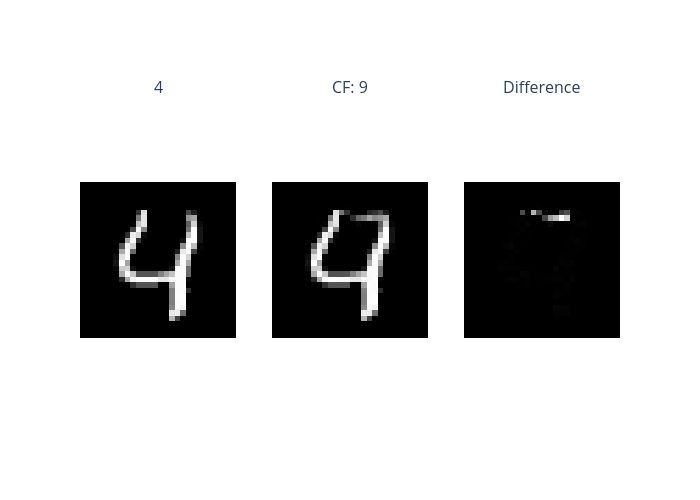
We can simply call explainer.explain to generate counterfactual examples for this classification task. ipython_plot plots the generated explanations in IPython. Parameter index indicates which instance to plot, e.g., index = 0 means plotting the first instance in test_imgs[0:5].

explanations = explainer.explain(test_imgs[0:5])
explanations.ipython_plot(index=4)

Binary step: 5 |███████████████████████████████████████-| 99.9%