PC algorithm for time series causal discovery

The Peter-Clark (PC) algorithm is one of the most general purpose algorithms for causal discovery that can be used for both tabular and time series data, of both continuous and discrete types. Briefly, the PC algorithm works in two steps, it first identifies the undirected causal graph, and then (partially) directs the edges. In the first step, we check for the existence of a causal connection between every pair of variables by checking if there exists a condition set (a subset of variables excluding the two said variables), conditioned on which, the two variables are independent. In the second step, the edges are directed by identifying colliders. Note that the edge orientation strategy of the PC algorithm may result in partially directed graphs. In the case of time series data, the additional information about the time steps associated with each variable can also be used to direct the edges.

The PC algorithm makes four core assumptions: 1. Causal Markov condition, which implies that two variables that are d-separated in a causal graph are probabilistically independent, 2. faithfulness, i.e., no conditional independence can hold unless the Causal Markov condition is met, 3. no hidden confounders, and 4. no cycles in the causal graph. 5. For time series data, it makes the additional assumption of stationarity, i.e., the properties of a. random variable is agnostic to the time step.

Finally, our current implementation of PC does not support contemporaneous causal links.

import numpy as np
import matplotlib
from matplotlib import pyplot as plt
%matplotlib inline
import pickle as pkl
import time

from causalai.models.time_series.pc import PCSingle, PC
from causalai.models.common.CI_tests.partial_correlation import PartialCorrelation
from causalai.models.common.CI_tests.kci import KCI
from causalai.data.data_generator import DataGenerator, GenerateRandomTimeseriesSEM
from causalai.models.common.CI_tests.discrete_ci_tests import DiscreteCI_tests


# also importing data object, data transform object, and prior knowledge object, and the graph plotting function
from causalai.data.time_series import TimeSeriesData
from causalai.data.transforms.time_series import StandardizeTransform
from causalai.models.common.prior_knowledge import PriorKnowledge
from causalai.misc.misc import plot_graph, get_precision_recall

Load and Visualize Data

Load the dataset and visualize the ground truth causal graph. For the purpose of this example, we will use a synthetic dataset available in our repository.

# fn = lambda x:x
# coef = 0.1
# sem = {
#         'a': [],
#         'b': [(('a', -1), coef, fn), (('f', -1), coef, fn)],
#         'c': [(('b', -2), coef, fn), (('f', -2), coef, fn)],
#         'd': [(('b', -4), coef, fn), (('b', -1), coef, fn), (('g', -1), coef, fn)],
#         'e': [(('f', -1), coef, fn)],
#         'f': [],
#         'g': [],
#         }

T = 5000

var_names = [str(i) for i in range(6)]
sem = GenerateRandomTimeseriesSEM(var_names=var_names, max_num_parents=2, seed=1)

data_array, var_names, graph_gt = DataGenerator(sem, T=T, seed=0)
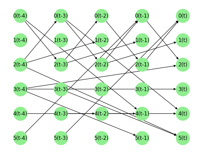
graph_gt

{'0': [('5', -3), ('2', -1)],
 '1': [('2', -2)],
 '2': [('3', -4), ('0', -1)],
 '3': [('3', -4)],
 '4': [('4', -2), ('0', -3)],
 '5': [('3', -3), ('2', -4)]}

Now we perform the following operations: 1. Standardize the data arrays 2. Create the data object

# 1.
StandardizeTransform_ = StandardizeTransform()
StandardizeTransform_.fit(data_array)

data_trans = StandardizeTransform_.transform(data_array)

# 2.
data_obj = TimeSeriesData(data_trans, var_names=var_names)

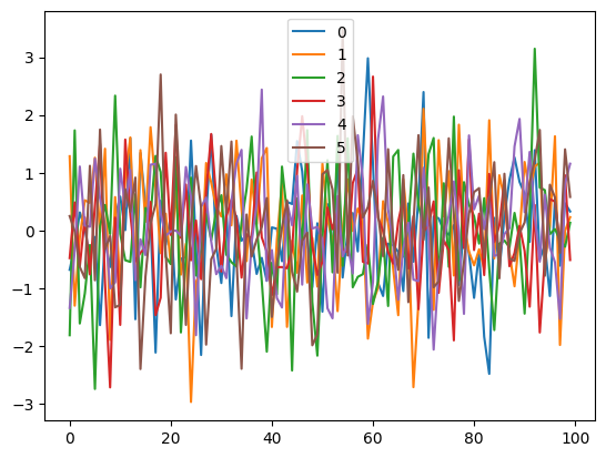
We visualize the data and graph below:

plot_graph(graph_gt, node_size=1000)



for i, n in enumerate(var_names):
    plt.plot(data_trans[-100:,i], label=n)
plt.legend()
plt.legend()
plt.show()

Causal Discovery (CD)

Our library supports running Granger causal discovery in two modes:

1. Targeted CD: Find causal parents of a single given variable. This is useful when we are only interested in finding out the cause of a specific variable, and not others. We thus save both compute and time this way.

2. Full CD: Find the full causal graph. This is costlier and scales linearly with the number of variables compared to the time taken by the mode above.

Enable/Disable Parallel Processing:

When we instantiate our causal discovery model, we need to decide if we want to use multi-processing. Multi-processing typically provides a significant speed-up for the PC algorithm. In order to use multi-processing in our causal discovery library, we pass the argument use_multiprocessing=True to the model constructor. It’s default value is False.

When running the PC algorithm in either of the above configurations, there is an optional functionality to enable a greedy heuristic that provides a further speed-up. More details are provided below in the Greedy Heuristic section.

Targeted Causal Discovery

prior_knowledge = None # PriorKnowledge(forbidden_links={'C': ['A']})

target_var = '0' # 'c'
max_lag = 5
pvalue_thres = 0.001#0.000000001
print(f'Target Variable: {target_var}, using max_lag {max_lag}, pvalue_thres {pvalue_thres}')

CI_test = PartialCorrelation() # use KCI() if the causal relationship is expected to be non-linear
# CI_test = KCI()
pc_single = PCSingle(
    data=data_obj,
    prior_knowledge=prior_knowledge,
    CI_test=CI_test,
    use_multiprocessing=False
    )

Target Variable: 0, using max_lag 5, pvalue_thres 0.001

tic = time.time()
result = pc_single.run(target_var=target_var, pvalue_thres=pvalue_thres, max_lag=max_lag, max_condition_set_size=None)

toc = time.time()
print(f'Time taken: {toc-tic:.2f}s\n')

for key in result.keys():
    print(key, '\n', result[key])
    print()

Time taken: 0.15s

parents
 [('5', -3), ('2', -1)]

value_dict
 {('0', -1): 0.008617392491692836, ('0', -2): 0.0018719655352873257, ('0', -3): -0.018247310621102835, ('0', -4): -0.008172415285694823, ('0', -5): -0.022965949303747218, ('1', -1): 0.0065014703986125445, ('1', -2): 0.0054060589346605565, ('1', -3): 0.010927859638999218, ('1', -4): 0.018428080161603726, ('1', -5): -0.004880797801728776, ('2', -1): 0.07966085711107593, ('2', -2): 0.020003191601610463, ('2', -3): -0.010856883544675107, ('2', -4): 0.005053791802773835, ('2', -5): -0.0011014065390646153, ('3', -1): 0.03805532987698295, ('3', -2): -0.019954514609284667, ('3', -3): -0.0013006743749435922, ('3', -4): 0.001083817267272737, ('3', -5): -0.00631117812741271, ('4', -1): 0.004332264603256165, ('4', -2): 0.0030765021801625668, ('4', -3): 0.022561445613761433, ('4', -4): 0.002766552799842021, ('4', -5): -0.018253328570831766, ('5', -1): -0.021362902145286, ('5', -2): 0.012457248161551112, ('5', -3): 0.10487138358725479, ('5', -4): -0.03378770240873199, ('5', -5): 0.00949296311111276}

pvalue_dict
 {('0', -1): 0.5437681136635399, ('0', -2): 0.895076012354255, ('0', -3): 0.1985587454758103, ('0', -4): 0.564768268966926, ('0', -5): 0.10561669473008387, ('1', -1): 0.6469185611842226, ('1', -2): 0.7032989349892531, ('1', -3): 0.44135104324767815, ('1', -4): 0.19414737580413452, ('1', -5): 0.7309481459822311, ('2', -1): 1.8962443807433843e-08, ('2', -2): 0.15871453292040036, ('2', -3): 0.44432340441297347, ('2', -4): 0.7218011906486563, ('2', -5): 0.9381490743831484, ('3', -1): 0.0073172562883217565, ('3', -2): 0.15973075647087706, ('3', -3): 0.9269878081050825, ('3', -4): 0.9391348897986946, ('3', -5): 0.6565797527269087, ('4', -1): 0.7601996508647306, ('4', -2): 0.8284058391576121, ('4', -3): 0.11190158349255867, ('4', -4): 0.845463515470323, ('4', -5): 0.19841071860251203, ('5', -1): 0.13226409935674308, ('5', -2): 0.3801209352060546, ('5', -3): 1.2740205766545935e-13, ('5', -4): 0.017261269740706457, ('5', -5): 0.503613902301266}

undirected_edges
 []

The output variable result is a dictionary with 3 keys, parents, value_dict and pvalue_dict. The first one is a list of the causal parents. Each of latter ones is a dictionary, with keys equal to all possile candidates of the specified target variable. On a side note, note that if any links are specified as forbidden in prior_knowledge, they will be ignored during the computation and will not be present in result.

The dictionary result['value_dict'] contains the strength of the link between the targeted variable and each of the candidate parents. The dictionary result['pvalue_dict'] contains the p-values of the said strength.

print(f'Predicted parents:')
parents = result['parents']
print(parents)

print(f"Ground truth parents:")
print(graph_gt[target_var])

Predicted parents:
[('5', -3), ('2', -1)]
Ground truth parents:
[('5', -3), ('2', -1)]

The way to read this Python dictionary is that \(0[t]\) has parents \(5[t-3]\) and \(2[t-1]\).

Full Causal Discovery

prior_knowledge = None #  PriorKnowledge(forbidden_links={})

max_lag = 5
pvalue_thres = 0.001
print(f'Using max_lag {max_lag}')
CI_test = PartialCorrelation()
# CI_test = KCI(chunk_size=100) # use if the causal relationship is expected to be non-linear
pc = PC(
        data=data_obj,
        prior_knowledge=prior_knowledge,
        CI_test=CI_test,
        use_multiprocessing=False
        )

Using max_lag 5

tic = time.time()


result = pc.run(pvalue_thres=pvalue_thres, max_lag=max_lag)

toc = time.time()
print(f'Time taken: {toc-tic:.2f}s\n')

Time taken: 0.73s

The output result now has the variable names as its keys, and the value corresponding to each key has the same format as the output of pc_single.run() example above for targeted CD.

print(f'Predicted parents:')
graph_est={n:[] for n in result.keys()}
for key in result.keys():
    parents = result[key]['parents']
    graph_est[key].extend(parents)
    print(f'{key}: {parents}')

print(f"\nGround truth parents:")
for key in graph_gt.keys():
    print(f'{key}: {graph_gt[key]}')

precision, recall, f1_score = get_precision_recall(graph_est, graph_gt)
print(f'Precision {precision:.2f}, Recall: {recall:.2f}, F1 score: {f1_score:.2f}')

Predicted parents:
0: [('5', -3), ('2', -1)]
1: [('2', -2)]
2: [('3', -4), ('0', -1)]
3: [('3', -4)]
4: [('0', -3), ('4', -2)]
5: [('2', -4), ('3', -3)]

Ground truth parents:
0: [('5', -3), ('2', -1)]
1: [('2', -2)]
2: [('3', -4), ('0', -1)]
3: [('3', -4)]
4: [('4', -2), ('0', -3)]
5: [('3', -3), ('2', -4)]
Precision 1.00, Recall: 1.00, F1 score: 1.00

The way to read this Python dictionary is that \(0[t]\) has parents \(5[t-3]\) and \(2[t-1]\), and so on.

Greedy Heuristic when the underlying true causal graph is sparse

When running the PC algorithm in either of the above configurations, enabling the greedy heuristic provides a speed-up on top of multi-processing.

The exact algorithm can be understood by looking through the run_greedy() in pc.py. In a nut shell, this procedure tries to determine the causal link between two variables by greedily conditioning on a condition set of increasing size, from 0 to the maximum number of possible parents or max_condition_set_size (whichever is lower). At each step, it permanently eliminates variables in the condition set whose causal strength is less than a specified value (determined by the pvalue_thres). Once all combinations of nodes are used as condition sets until max_condition_set_size, it then uses all the variables (except those that got eliminated, and the 2 variables being check) as the condition set. This step helps remove edges for which the condition set is larger than max_condition_set_size.

Using this greedy heuristic can significantly speed-up the algorithm when the underlying true causal graph is sparse because most of the candidate parents for each variable get eliminated in the greedy step with a relatively small computational cost.

An example for the single target variable case is given below. The only additional argument that needs to be passed is max_condition_set_size. The full causal discovery algorithm can be called similarly with the same additional argument max_condition_set_size.

We compare the time taken by the PC algorithm with and without the greedy heuristic. To make the difference in time taken apparent, we set max_lag=30, which makes the effective number of variables = 6x30=180.

T = 5000

var_names = ['a','b','c','d','e','f']
sem = GenerateRandomTimeseriesSEM(var_names=var_names, max_num_parents=2, seed=1)

data_array, var_names, graph_gt = DataGenerator(sem, T=T, seed=0)


StandardizeTransform_ = StandardizeTransform()
StandardizeTransform_.fit(data_array)
data_trans = StandardizeTransform_.transform(data_array)
data_obj = TimeSeriesData(data_trans, var_names=var_names)



prior_knowledge = None # PriorKnowledge(forbidden_links={'b': ['c']})

target_var = 'c'
max_lag = 30
print(f'Target Variable: {target_var}, using max_lag {max_lag}')

Target Variable: c, using max_lag 30

print(f"Ground truth parents for target variable {target_var}:")
print(graph_gt[target_var])
print('\n')

# without greedy heuristic

CI_test = PartialCorrelation()
pc_single = PCSingle(
    data=data_obj,
    prior_knowledge=prior_knowledge,
    CI_test=CI_test,
    use_multiprocessing=True
    )

tic = time.time()
result = pc_single.run(target_var=target_var, pvalue_thres=0.01, max_lag=max_lag, max_condition_set_size=None)

toc = time.time()
print(f'Time taken without greedy heuristic: {toc-tic:.2f}s')
print(f'Predicted parents without greedy heuristic:')
parents = result['parents']
print(parents)
print('\n')


# with greedy heuristic

CI_test = PartialCorrelation()
pc_single = PCSingle(
    data=data_obj,
    prior_knowledge=prior_knowledge,
    CI_test=CI_test,
    use_multiprocessing=True
    )

tic = time.time()

result = pc_single.run(target_var=target_var, pvalue_thres=0.01, max_lag=max_lag, max_condition_set_size=2)

toc = time.time()
print(f'Time taken with greedy heuristic: {toc-tic:.2f}s')
print(f'Predicted parents with greedy heuristic:')
parents = result['parents']
print(parents)

Ground truth parents for target variable c:
[('d', -4), ('a', -1)]

2023-08-17 07:38:31,943 INFO worker.py:1553 -- Started a local Ray instance.

Time taken without greedy heuristic: 28.82s
Predicted parents without greedy heuristic:
[('d', -4), ('a', -1), ('c', -17)]

2023-08-17 07:39:01,090 INFO worker.py:1553 -- Started a local Ray instance.

Time taken with greedy heuristic: 11.91s
Predicted parents with greedy heuristic:
[('d', -4), ('a', -1), ('c', -17)]

The way to read this Python dictionary is that \(c[t]\) has parents \(d[t-4]\) and \(a[t-1]\). Note that the greedy heuristic takes less time.