PC Algorithm for Tabular Causal Discovery
The Peter-Clark (PC) algorithm is one of the most general purpose algorithms for causal discovery that can be used for both tabular and time series data, of both continuous and discrete types. Briefly, the PC algorithm works in two steps, it first identifies the undirected causal graph, and then (partially) directs the edges. In the first step, we check for the existence of a causal connection between every pair of variables by checking if there exists a condition set (a subset of variables excluding the two said variables), conditioned on which, the two variables are independent. In the second step, the edges are directed by identifying colliders. Note that the edge orientation strategy of the PC algorithm may result in partially directed graphs.
The PC algorithm makes four core assumptions: 1. Causal Markov condition, which implies that two variables that are d-separated in a causal graph are probabilistically independent, 2. faithfulness, i.e., no conditional independence can hold unless the Causal Markov condition is met, 3. no hidden confounders, and 4. no cycles in the causal graph.
Edge Orientation
Note that the causal edge orientation module of the tabular PC algorithm can yield quite inaccurate results in some cases. Nonetheless, the causal graph skeleton (i.e., the undirected graph) is often quite accurate. We discuss this below as well.
[1]:
import numpy as np
import matplotlib
from matplotlib import pyplot as plt
%matplotlib inline
import pickle as pkl
import time
[2]:
from causalai.models.tabular.pc import PCSingle, PC
from causalai.models.common.CI_tests.partial_correlation import PartialCorrelation
from causalai.models.common.CI_tests.discrete_ci_tests import DiscreteCI_tests
from causalai.models.common.CI_tests.kci import KCI


# also importing data object, data transform object, and prior knowledge object, and the graph plotting function
from causalai.data.data_generator import DataGenerator, GenerateRandomTabularSEM
from causalai.data.tabular import TabularData
from causalai.data.transforms.time_series import StandardizeTransform
from causalai.models.common.prior_knowledge import PriorKnowledge
from causalai.misc.misc import plot_graph, get_precision_recall, get_precision_recall_skeleton, make_symmetric
Load and Visualize Data
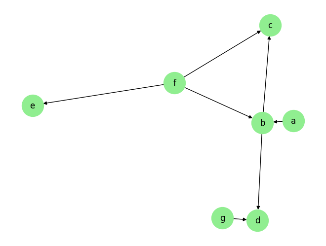
Load the dataset and visualize the ground truth causal graph. For the purpose of this example, we will use a synthetic dataset available in our repository.
[3]:
fn = lambda x:x
coef = 0.1
sem = {
        'a': [],
        'b': [('a', coef, fn), ('f', coef, fn)],
        'c': [('b', coef, fn), ('f', coef, fn)],
        'd': [('b', coef, fn), ('g', coef, fn)],
        'e': [('f', coef, fn)],
        'f': [],
        'g': [],
        }
T = 5000

# var_names = [str(i) for i in range(5)]
# sem = GenerateRandomTabularSEM(var_names=var_names, max_num_parents=2, seed=1)
data_array, var_names, graph_gt = DataGenerator(sem, T=T, seed=0, discrete=False)

graph_gt
[3]:
{'a': [],
 'b': ['a', 'f'],
 'c': ['b', 'f'],
 'd': ['b', 'g'],
 'e': ['f'],
 'f': [],
 'g': []}
Now we perform the following operations: 1. Standardize the data arrays 2. Create the data object
[4]:
# 1.
StandardizeTransform_ = StandardizeTransform()
StandardizeTransform_.fit(data_array)

data_trans = StandardizeTransform_.transform(data_array)

# 2.
data_obj = TabularData(data_trans, var_names=var_names)
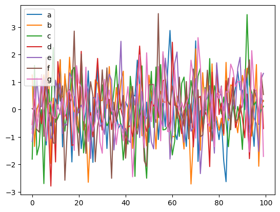
We visualize the data and graph below:
[5]:
plot_graph(graph_gt, node_size=1000)


for i, n in enumerate(var_names):
    plt.plot(data_trans[-100:,i], label=n)
plt.legend()
plt.legend()
plt.show()
Causal Discovery (CD)
Enable/Disable Multi-Processing:
When we instantiate our causal discovery model, we need to decide if we want to use multi-processing. Multi-processing typically provides a significant speed-up for the PC algorithm. In order to use multi-processing in our causal discovery library, we pass the argument use_multiprocessing=True to the model constructor. It’s default value is False.
Note that for tabular PC, we do not support targeted causal discovery as in the time series case. We only support full causal discovery.
Full Causal Discovery
[6]:
prior_knowledge = None #  PriorKnowledge(forbidden_links={'a': ['b']})

pvalue_thres = 0.01
CI_test = PartialCorrelation()
# CI_test = KCI(chunk_size=100) # use if the causal relationship is expected to be non-linear
pc = PC(
        data=data_obj,
        prior_knowledge=prior_knowledge,
        CI_test=CI_test,
        use_multiprocessing=False
        )
[7]:
tic = time.time()


result = pc.run(pvalue_thres=pvalue_thres, max_condition_set_size=2)

toc = time.time()

print(f'Time taken: {toc-tic:.2f}s\n')

print(f' The output result has keys: {result.keys()}')
print(f' The output result["a"] has keys: {result["a"].keys()}')
Time taken: 0.10s

 The output result has keys: dict_keys(['a', 'b', 'c', 'd', 'e', 'f', 'g'])
 The output result["a"] has keys: dict_keys(['parents', 'value_dict', 'pvalue_dict'])
The output result has the variable names as its keys, and the value corresponding to each key is a dictionary with 3 keys, parents, value_dict and pvalue_dict. The first one is a list of the causal parents. The dictionary result['value_dict'] contains the strength of the link between the targeted variable and each of the candidate parents. The dictionary result['pvalue_dict'] contains the p-values of the said strength.
[8]:
print(f'Predicted parents:')

graph_est={n:[] for n in result.keys()}
for key in result.keys():
    parents = result[key]['parents']
    graph_est[key].extend(parents)
    print(f'{key}: {parents}')
print()

print(f"\nGround truth parents:")
for key in graph_gt.keys():
    print(f'{key}: {graph_gt[key]}')

precision, recall, f1_score = get_precision_recall(graph_est, graph_gt)
print(f'Precision {precision:.2f}, Recall: {recall:.2f}, F1 score: {f1_score:.2f}')
Predicted parents:
a: ['b']
b: ['d', 'c', 'f', 'a']
c: ['f', 'b']
d: ['g', 'b']
e: ['f']
f: ['e', 'c', 'b']
g: ['d']


Ground truth parents:
a: []
b: ['a', 'f']
c: ['b', 'f']
d: ['b', 'g']
e: ['f']
f: []
g: []
Precision 0.50, Recall: 1.00, F1 score: 0.52
Edge Orientation
As we mentioned at the beginning, the causal edge orientation module (which relies on colliders) of the tabular PC algorithm can yield quite inaccurate results in some cases. In general, we find that for tabular data, edge orientation in the causal discovery process is not as reliable as that in the case of time series data. This is because in time series, edges always go from past to future. But such information is absent in tabular data, which makes the edge orintation problem harder.
Nonetheless, we find that the undirected version of the estimated causal graph (aka skeleton), is much more accurate. To get the discovered skeleton instead of the directed graph, there is a skeleton attribute which can be called as follows. Alternatively, one can also use make_symmetric(graph_est).
Below, we find that the estimated undirected causal graph has much higher/perfect precision recall compared with the ground truth undirected causal graph.
[9]:
pc.skeleton # can also use make_symmetric(graph_est)
[9]:
{'a': ['b'],
 'b': ['c', 'd', 'f', 'a'],
 'c': ['b', 'f'],
 'd': ['b', 'g'],
 'e': ['f'],
 'f': ['e', 'c', 'b'],
 'g': ['d']}
Here the value correcponding to each key (node) is a list of all the connected nodes, which could be either parents of children.
Now, to evaluate the correctness of the estimated undirected causal graph (skeleton), we can call the get_precision_recall_undirected function as follows,
[10]:
print(f"\nGround truth skeleton:")
graph_gt_symm = make_symmetric(graph_gt)
for key in graph_gt_symm.keys():
    print(f'{key}: {graph_gt_symm[key]}')

print(f"\n Est skeleton:")
for key in pc.skeleton.keys():
    print(f'{key}: {pc.skeleton[key]}')

precision, recall, f1_score = get_precision_recall_skeleton(pc.skeleton, graph_gt)
print(f'Precision {precision:.2f}, Recall: {recall:.2f}, F1 score: {f1_score:.2f}')
Ground truth skeleton:
a: ['b']
b: ['a', 'f', 'c', 'd']
c: ['b', 'f']
d: ['b', 'g']
e: ['f']
f: ['b', 'c', 'e']
g: ['d']

 Est skeleton:
a: ['b']
b: ['c', 'd', 'f', 'a']
c: ['b', 'f']
d: ['b', 'g']
e: ['f']
f: ['e', 'c', 'b']
g: ['d']
Precision 1.00, Recall: 1.00, F1 score: 1.00
Causal Discovery for Discrete Data
[11]:
fn = lambda x:x
coef = 0.1
sem = {
        'a': [],
        'b': [('a', coef, fn), ('f', coef, fn)],
        'c': [('b', coef, fn), ('f', coef, fn)],
        'd': [('b', coef, fn), ('g', coef, fn)],
        'e': [('f', coef, fn)],
        'f': [],
        'g': [],
        }
T = 5000
data_array, var_names, graph_gt = DataGenerator(sem, T=T, seed=0, discrete=True)

plot_graph(graph_gt, node_size=200)
graph_gt
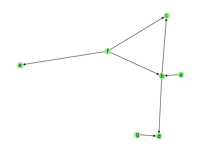
[11]:
{'a': [],
 'b': ['a', 'f'],
 'c': ['b', 'f'],
 'd': ['b', 'g'],
 'e': ['f'],
 'f': [],
 'g': []}
[12]:
data_obj = TabularData(data_array, var_names=var_names)
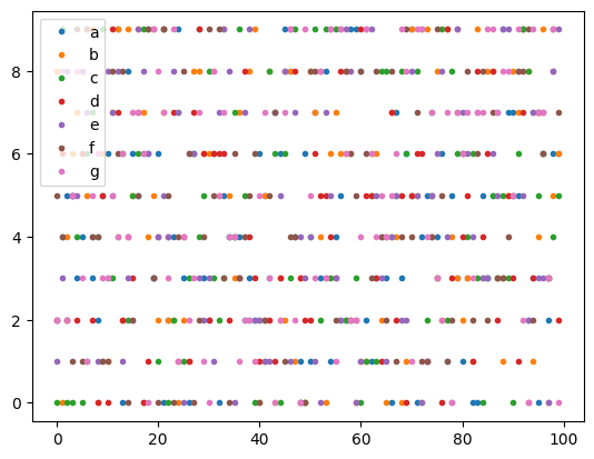
[13]:
for i, n in enumerate(var_names):
    plt.plot(data_array[-100:,i], '.', label=n)
plt.legend()
plt.legend()
plt.show()
[14]:
prior_knowledge =None# PriorKnowledge(forbidden_links={'c': ['e']}) # g cannot be a parent of c

pvalue_thres = 0.05
CI_test = DiscreteCI_tests(method="pearson")
pc = PC(
        data=data_obj,
        prior_knowledge=prior_knowledge,
        CI_test=CI_test,
        use_multiprocessing=False
        )

tic = time.time()

result = pc.run(pvalue_thres=pvalue_thres, max_condition_set_size=3)

toc = time.time()

print(f'Time taken: {toc-tic:.2f}s\n')
Time taken: 0.31s
[15]:
print(f'Predicted parents:')

graph_est={n:[] for n in result.keys()}
for key in result.keys():
    parents = result[key]['parents']
    graph_est[key].extend(parents)
    print(f'{key}: {parents}')
print()

print(f"\nGround truth parents:")
for key in graph_gt.keys():
    print(f'{key}: {graph_gt[key]}')

precision, recall, f1_score = get_precision_recall(graph_est, graph_gt)
print(f'Precision {precision:.2f}, Recall: {recall:.2f}, F1 score: {f1_score:.2f}')
Predicted parents:
a: ['b']
b: ['a']
c: []
d: ['g']
e: ['f']
f: ['e']
g: ['d']


Ground truth parents:
a: []
b: ['a', 'f']
c: ['b', 'f']
d: ['b', 'g']
e: ['f']
f: []
g: []
Precision 0.43, Recall: 0.71, F1 score: 0.33
Here the value correcponding to each key (node) is a list of all the connected nodes, which could be either parents of children.
Now, to evaluate the correctness of the estimated undirected causal graph (skeleton), we can call the get_precision_recall_undirected function as follows,
[16]:
print(f"\nGround truth skeleton:")
graph_gt_symm = make_symmetric(graph_gt)
for key in graph_gt_symm.keys():
    print(f'{key}: {graph_gt_symm[key]}')

print(f"\nEst skeleton:")
for key in pc.skeleton.keys():
    print(f'{key}: {pc.skeleton[key]}')

precision, recall, f1_score = get_precision_recall_skeleton(pc.skeleton, graph_gt)
print(f'Precision {precision:.2f}, Recall: {recall:.2f}, F1 score: {f1_score:.2f}')
Ground truth skeleton:
a: ['b']
b: ['a', 'f', 'c', 'd']
c: ['b', 'f']
d: ['b', 'g']
e: ['f']
f: ['b', 'c', 'e']
g: ['d']

Est skeleton:
a: ['b']
b: []
c: []
d: []
e: ['f']
f: []
g: ['d']
Precision 0.86, Recall: 0.58, F1 score: 0.65
Prior Knowledge Usage
[11]:
fn = lambda x:x
coef = 0.1
sem = {
        'a': [],
        'b': [('a', coef, fn), ('f', coef, fn)],
        'c': [('b', coef, fn), ('f', coef, fn)],
        'd': [('b', coef, fn), ('g', coef, fn)],
        'e': [('f', coef, fn)],
        'f': [],
        'g': [],
        }
T = 5000

# var_names = [str(i) for i in range(5)]
# sem = GenerateRandomTabularSEM(var_names=var_names, max_num_parents=2, seed=1)
data_array, var_names, graph_gt = DataGenerator(sem, T=T, seed=0, discrete=False)

graph_gt
[11]:
{'a': [],
 'b': ['a', 'f'],
 'c': ['b', 'f'],
 'd': ['b', 'g'],
 'e': ['f'],
 'f': [],
 'g': []}
[12]:
# 1.
StandardizeTransform_ = StandardizeTransform()
StandardizeTransform_.fit(data_array)

data_trans = StandardizeTransform_.transform(data_array)

# 2.
data_obj = TabularData(data_trans, var_names=var_names)
Without Prior Knowledge
[13]:
prior_knowledge = None #  PriorKnowledge(forbidden_links={'a': ['b']})

pvalue_thres = 0.01
CI_test = PartialCorrelation()
# CI_test = KCI(chunk_size=100) # use if the causal relationship is expected to be non-linear
pc = PC(
        data=data_obj,
        prior_knowledge=prior_knowledge,
        CI_test=CI_test,
        use_multiprocessing=False
        )

tic = time.time()


result = pc.run(pvalue_thres=pvalue_thres, max_condition_set_size=2)

toc = time.time()

print(f'Time taken: {toc-tic:.2f}s\n')

print(f'Predicted parents:')

graph_est={n:[] for n in result.keys()}
for key in result.keys():
    parents = result[key]['parents']
    graph_est[key].extend(parents)
    print(f'{key}: {parents}')
print()

print(f"\nGround truth parents:")
for key in graph_gt.keys():
    print(f'{key}: {graph_gt[key]}')

precision, recall, f1_score = get_precision_recall(graph_est, graph_gt)
print(f'Precision {precision:.2f}, Recall: {recall:.2f}, F1 score: {f1_score:.2f}')
Time taken: 0.10s

Predicted parents:
a: ['b']
b: ['d', 'c', 'f', 'a']
c: ['f', 'b']
d: ['g', 'b']
e: ['f']
f: ['e', 'c', 'b']
g: ['d']


Ground truth parents:
a: []
b: ['a', 'f']
c: ['b', 'f']
d: ['b', 'g']
e: ['f']
f: []
g: []
Precision 0.50, Recall: 1.00, F1 score: 0.52
With Prior Knowledge: specifying forbidden links. Notice how the link b->a no longer appears in the estimated graph.
[14]:
prior_knowledge = PriorKnowledge(forbidden_links={'a': ['b']})

pvalue_thres = 0.01
CI_test = PartialCorrelation()
# CI_test = KCI(chunk_size=100) # use if the causal relationship is expected to be non-linear
pc = PC(
        data=data_obj,
        prior_knowledge=prior_knowledge,
        CI_test=CI_test,
        use_multiprocessing=False
        )

tic = time.time()


result = pc.run(pvalue_thres=pvalue_thres, max_condition_set_size=2)

toc = time.time()

print(f'Time taken: {toc-tic:.2f}s\n')

print(f'Predicted parents:')

graph_est={n:[] for n in result.keys()}
for key in result.keys():
    parents = result[key]['parents']
    graph_est[key].extend(parents)
    print(f'{key}: {parents}')
print()

print(f"\nGround truth parents:")
for key in graph_gt.keys():
    print(f'{key}: {graph_gt[key]}')

precision, recall, f1_score = get_precision_recall(graph_est, graph_gt)
print(f'Precision {precision:.2f}, Recall: {recall:.2f}, F1 score: {f1_score:.2f}')
Time taken: 0.10s

Predicted parents:
a: []
b: ['d', 'c', 'f', 'a']
c: ['f', 'b']
d: ['g', 'b']
e: ['f']
f: ['e', 'c', 'b']
g: ['d']


Ground truth parents:
a: []
b: ['a', 'f']
c: ['b', 'f']
d: ['b', 'g']
e: ['f']
f: []
g: []
Precision 0.64, Recall: 1.00, F1 score: 0.67
With Prior Knowledge: specifying existing links. Notice how the link a->b appears in the estimated graph, and b->a does not.
[15]:
prior_knowledge = PriorKnowledge(existing_links={'b': ['a']})

pvalue_thres = 0.01
CI_test = PartialCorrelation()
# CI_test = KCI(chunk_size=100) # use if the causal relationship is expected to be non-linear
pc = PC(
        data=data_obj,
        prior_knowledge=prior_knowledge,
        CI_test=CI_test,
        use_multiprocessing=False
        )

tic = time.time()


result = pc.run(pvalue_thres=pvalue_thres, max_condition_set_size=2)

toc = time.time()

print(f'Time taken: {toc-tic:.2f}s\n')

print(f'Predicted parents:')

graph_est={n:[] for n in result.keys()}
for key in result.keys():
    parents = result[key]['parents']
    graph_est[key].extend(parents)
    print(f'{key}: {parents}')
print()

print(f"\nGround truth parents:")
for key in graph_gt.keys():
    print(f'{key}: {graph_gt[key]}')

precision, recall, f1_score = get_precision_recall(graph_est, graph_gt)
print(f'Precision {precision:.2f}, Recall: {recall:.2f}, F1 score: {f1_score:.2f}')
Time taken: 0.11s

Predicted parents:
a: []
b: ['d', 'c', 'f', 'a']
c: ['f', 'b']
d: ['g', 'b']
e: ['f']
f: ['e', 'c', 'b']
g: ['d']


Ground truth parents:
a: []
b: ['a', 'f']
c: ['b', 'f']
d: ['b', 'g']
e: ['f']
f: []
g: []
Precision 0.64, Recall: 1.00, F1 score: 0.67
With Prior Knowledge: specifying root nodes. Notice how nodes a and f have no parents in the estimated graph.
[18]:
prior_knowledge = PriorKnowledge(root_variables=['a', 'f'])

pvalue_thres = 0.01
CI_test = PartialCorrelation()
# CI_test = KCI(chunk_size=100) # use if the causal relationship is expected to be non-linear
pc = PC(
        data=data_obj,
        prior_knowledge=prior_knowledge,
        CI_test=CI_test,
        use_multiprocessing=False
        )

tic = time.time()


result = pc.run(pvalue_thres=pvalue_thres, max_condition_set_size=2)

toc = time.time()

print(f'Time taken: {toc-tic:.2f}s\n')

print(f'Predicted parents:')

graph_est={n:[] for n in result.keys()}
for key in result.keys():
    parents = result[key]['parents']
    graph_est[key].extend(parents)
    print(f'{key}: {parents}')
print()

print(f"\nGround truth parents:")
for key in graph_gt.keys():
    print(f'{key}: {graph_gt[key]}')

precision, recall, f1_score = get_precision_recall(graph_est, graph_gt)
print(f'Precision {precision:.2f}, Recall: {recall:.2f}, F1 score: {f1_score:.2f}')
Time taken: 0.09s

Predicted parents:
a: []
b: ['d', 'c', 'f', 'a']
c: ['f', 'b']
d: ['g', 'b']
e: ['f']
f: []
g: ['d']


Ground truth parents:
a: []
b: ['a', 'f']
c: ['b', 'f']
d: ['b', 'g']
e: ['f']
f: []
g: []
Precision 0.79, Recall: 1.00, F1 score: 0.81
With Prior Knowledge: specifying leaf nodes. Notice how nodes d and c are never parents in the estimated graph.
[20]:
prior_knowledge = PriorKnowledge(leaf_variables=['d', 'c'])

pvalue_thres = 0.01
CI_test = PartialCorrelation()
# CI_test = KCI(chunk_size=100) # use if the causal relationship is expected to be non-linear
pc = PC(
        data=data_obj,
        prior_knowledge=prior_knowledge,
        CI_test=CI_test,
        use_multiprocessing=False
        )

tic = time.time()


result = pc.run(pvalue_thres=pvalue_thres, max_condition_set_size=2)

toc = time.time()

print(f'Time taken: {toc-tic:.2f}s\n')

print(f'Predicted parents:')

graph_est={n:[] for n in result.keys()}
for key in result.keys():
    parents = result[key]['parents']
    graph_est[key].extend(parents)
    print(f'{key}: {parents}')
print()

print(f"\nGround truth parents:")
for key in graph_gt.keys():
    print(f'{key}: {graph_gt[key]}')

precision, recall, f1_score = get_precision_recall(graph_est, graph_gt)
print(f'Precision {precision:.2f}, Recall: {recall:.2f}, F1 score: {f1_score:.2f}')
Time taken: 0.12s

Predicted parents:
a: ['b']
b: ['f', 'a']
c: ['f', 'b']
d: ['g', 'b']
e: ['f']
f: ['e', 'b']
g: []


Ground truth parents:
a: []
b: ['a', 'f']
c: ['b', 'f']
d: ['b', 'g']
e: ['f']
f: []
g: []
Precision 0.71, Recall: 1.00, F1 score: 0.71
[ ]: