GES for Tabular Causal Discovery

Greedy Equivalence Search (GES) heuristically searches the space of causal Bayesian network and returns the model with highest Bayesian score it finds. Specifically, GES starts its search with the empty graph. It then performs a forward search in which edges are added between nodes in order to increase the Bayesian score. This process is repeated until no single edge addition increases the score. Finally, it performs a backward search that removes edges until no single edge removal can increase the score.

This algorithm makes the following assumptions: 1. observational samples are i.i.d. 2. linear relationship between variables with Gaussian noise terms, 3. Causal Markov condition, which implies that two variables that are d-separated in a causal graph are probabilistically independent 4. faithfulness, i.e., no conditional independence can hold unless the Causal Markov condition is met, 5. no hidden confounders. We do not support multi-processing for this algorithm.

import numpy as np
import matplotlib
from matplotlib import pyplot as plt
%matplotlib inline
import pickle as pkl
import time

from causalai.models.tabular.ges import GES

from causalai.data.data_generator import DataGenerator
# also importing data object, data transform object, and prior knowledge object, and the graph plotting function
from causalai.data.tabular import TabularData
from causalai.data.transforms.tabular import StandardizeTransform
from causalai.models.common.prior_knowledge import PriorKnowledge
from causalai.misc.misc import plot_graph, get_precision_recall, get_precision_recall_skeleton, make_symmetric

Load and Visualize Data

Load the dataset and visualize the ground truth causal graph. For the purpose of this example, we will use a synthetic dataset available in our repository.

fn = lambda x:x
coef = 0.1
sem = {
        'a': [],
        'b': [('a', coef, fn), ('f', coef, fn)],
        'c': [('b', coef, fn), ('f', coef, fn)],
        'd': [('b', coef, fn), ('g', coef, fn)],
        'e': [('f', coef, fn)],
        'f': [],
        'g': [],
        }
T = 5000

# var_names = [str(i) for i in range(5)]
# sem = GenerateRandomTabularSEM(var_names=var_names, max_num_parents=2, seed=1)
data_array, var_names, graph_gt = DataGenerator(sem, T=T, seed=0, discrete=False)
# data_array = np.random.randn(T, 7) # load your own data
# var_names = ['a', 'b', 'c', 'd', 'e', 'f', 'g']

graph_gt

{'a': [],
 'b': ['a', 'f'],
 'c': ['b', 'f'],
 'd': ['b', 'g'],
 'e': ['f'],
 'f': [],
 'g': []}

Now we perform the following operations:

1. Standardize the data arrays

2. Create the data object

# 1.
StandardizeTransform_ = StandardizeTransform()
StandardizeTransform_.fit(data_array)

data_trans = StandardizeTransform_.transform(data_array)

# 2.
data_obj = TabularData(data_trans, var_names=var_names)

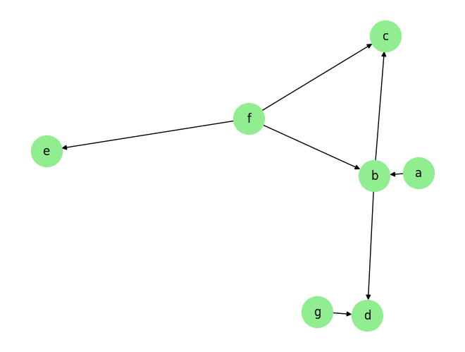
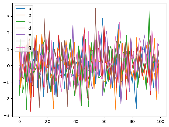
We visualize the data and graph below:

plot_graph(graph_gt, node_size=1000)



for i, n in enumerate(var_names):
    plt.plot(data_trans[-100:,i], label=n)
plt.legend()
plt.legend()
plt.show()

Causal Discovery (CD)

For GES algorithm, causal discovery can be performed for the whole graph (Full Causal Discovery). Targeted causal discovery (finding parents of a specific target variable) is not supported like some of the other algorithms in our library.

Multiprocessing is not supported in GES.

Prior Knowledge is supported in GES.

Full Causal Discovery

prior_knowledge = None #  PriorKnowledge(forbidden_links={'f': ['e']})

ges = GES(
        data=data_obj,
        prior_knowledge=prior_knowledge
        )

tic = time.time()
result = ges.run()
toc = time.time()
print(f'Time taken: {toc-tic:.2f}s\n')


print(f' The output result has keys: {result.keys()}')
print(f' The output result["a"] has keys: {result["a"].keys()}')

Time taken: 0.10s

 The output result has keys: dict_keys(['a', 'b', 'c', 'd', 'e', 'f', 'g'])
 The output result["a"] has keys: dict_keys(['value_dict', 'pvalue_dict', 'parents'])

The output result has the variable names as its keys, and the value corresponding to each key is a dictionary with 3 keys, parents, value_dict and pvalue_dict. The first one is a list of the causal parents. The dictionary result['value_dict'] contains the strength of the link between the targeted variable and each of the candidate parents. The dictionary result['pvalue_dict'] contains the p-values of the said strength.

print(f'Predicted parents:')
graph_est={n:[] for n in result.keys()}
for key in result.keys():
    parents = result[key]['parents']
    graph_est[key].extend(parents)
    print(f'{key}: {parents}')

print(f"\nGround truth parents:")
for key in graph_gt.keys():
    print(f'{key}: {graph_gt[key]}')

precision, recall, f1_score = get_precision_recall(graph_est, graph_gt)
print(f'Precision {precision:.2f}, Recall: {recall:.2f}, F1 score: {f1_score:.2f}')

Predicted parents:
a: []
b: ['a', 'd']
c: ['b', 'f']
d: ['g']
e: []
f: ['b', 'e']
g: ['d']

Ground truth parents:
a: []
b: ['a', 'f']
c: ['b', 'f']
d: ['b', 'g']
e: ['f']
f: []
g: []
Precision 0.50, Recall: 0.71, F1 score: 0.45

In general, we find that for tabular data, edge orientation in the causal discovery process is not as reliable as that in the case of time series data. This is because in time series, edges always go from past to future. But such information is absent in tabular data, which makes the edge orintation problem harder.

Nonetheless, we find that the undirected version of the estimated causal graph (aka skeleton), is much more accurate. The undirected graph can be obtained from the estimated directed causal graph by simply making the graph edges symmetric.

Below, we find that the estimated undirected causal graph has much higher/perfect precision recall compared with the ground truth undirected causal graph.

print(f"\nGround truth skeleton:")
graph_gt_symm = make_symmetric(graph_gt)
for key in graph_gt_symm.keys():
    print(f'{key}: {graph_gt_symm[key]}')

print(f"\n Est skeleton:")
graph_est_symm = make_symmetric(graph_est)
for key in graph_est_symm.keys():
    print(f'{key}: {graph_est_symm[key]}')

precision, recall, f1_score = get_precision_recall_skeleton(graph_est, graph_gt)
print(f'Precision {precision:.2f}, Recall: {recall:.2f}, F1 score: {f1_score:.2f}')

Ground truth skeleton:
a: ['b']
b: ['a', 'f', 'c', 'd']
c: ['b', 'f']
d: ['b', 'g']
e: ['f']
f: ['b', 'c', 'e']
g: ['d']

 Est skeleton:
a: ['b']
b: ['a', 'd', 'c', 'f']
c: ['b', 'f']
d: ['b', 'g']
e: ['f']
f: ['c', 'b', 'e']
g: ['d']
Precision 1.00, Recall: 1.00, F1 score: 1.00